First Modeling Steps
Simple Duct with Intake Cylinder
This tutorial is a good starting point for CAESES. It shows you basic modeling techniques and introduces the modeling concept of CAESES. As an example, a simple parametric duct is created.
As a prerequisite we recommend watching the introduction videos to get familiar with the graphical user interface.
CAESES Video Portal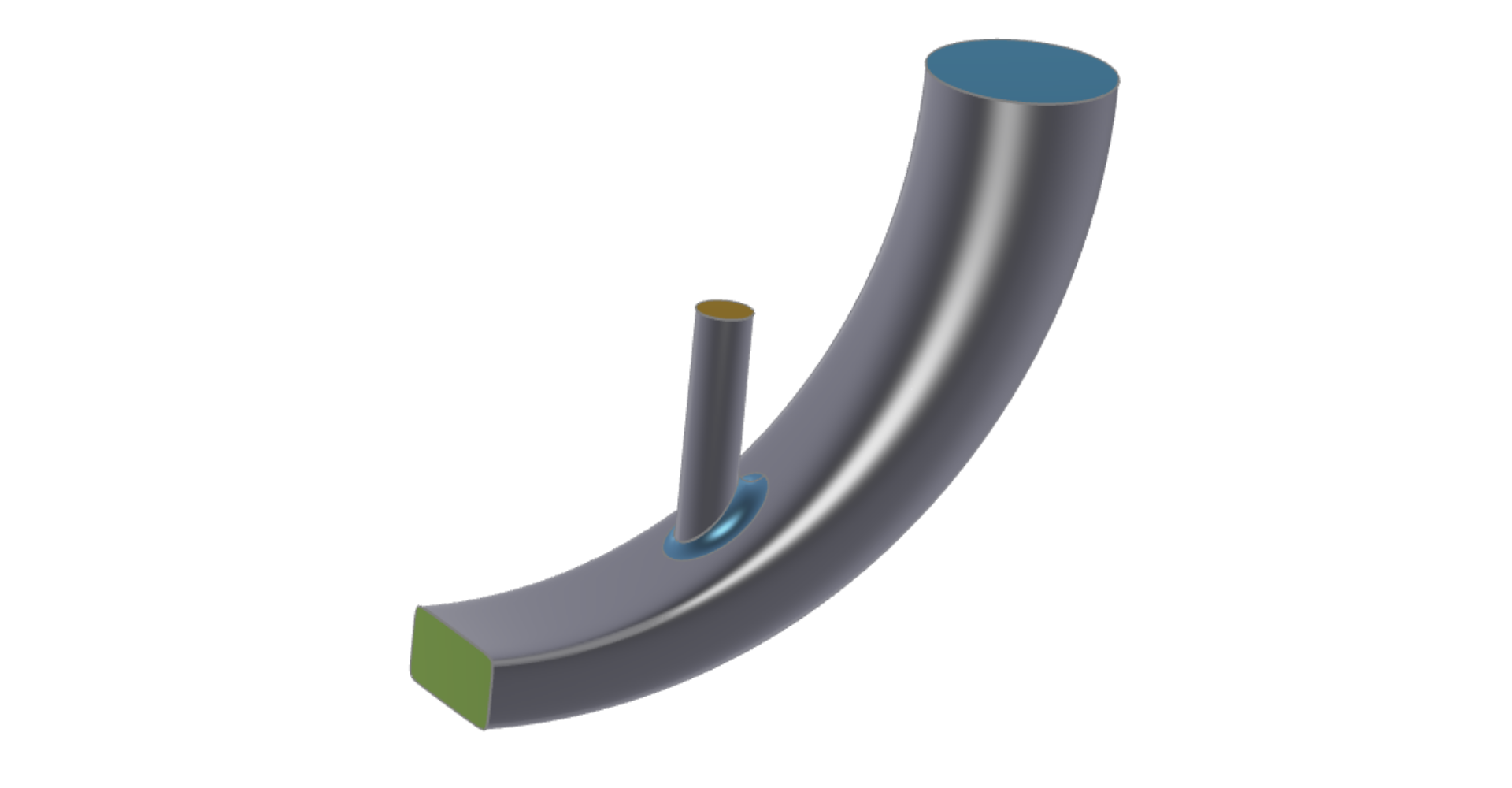
After this tutorial, you will have a basic understanding of how to create parameterized geometries including curves, surfaces and solid bodies, which can later be used for automatic generation of design variants, CFD integration and design optimization.
If you prefer watching a video, this tutorial is also available as a video tutorial:
Watch Tutorial VideoCenterline
In this first step we will define the centerline of the duct. We will create this curve in the XY-plane.
- Save your project first via Menu > File > Save Project As.
You can also use the standard short cuts for saving (Ctrl + S) or opening (Ctrl + O) projects or you can use the quick action buttons in the blue title bar.
- Set the orientation of the XY-plane by clicking on the Z-face of the 3D navigation cube, or chose the Z-(X,Y) plane from the views menu:

- Set the workspace with the left navigation bar to Model.
With the left side/navigation bar you can cycle through different workspaces.
Inside each workspace you can find tabs, which you can change within the blue title bar. Each tab will have a ribbon toolbar below it, which contains objects or commands.
For more information please have a look at the introduction of the GUI inside the CAESES documentation.
- Create a scope via Model > CAD > Scope and set the name to "01_centerline".
- Click with the middle mouse button on this scope to make it a working scope.
When a working scope is active, then each new object will be created inside this scope. You can activate or deactivate it with the middle mouse button or via the context menu.
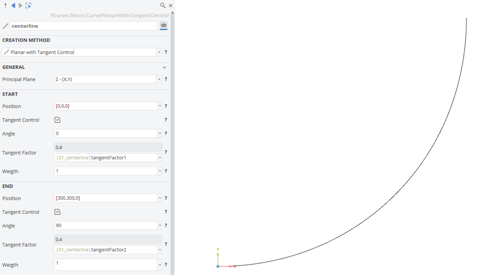
- Create a curve via Model > CAD > Curves > Point Based > Planar with Tangent Control and set the name to "centerline".
This curve is internally a NURBS curve with two control points between the start and the end. This makes the curve quite flexible to set tangent angles, speeds and weights.
- Set the Start Tangent Factor to
0.4. - Set the End Position to
[300,300,0]. - Click on the Reset Zoom button to fit the view:

- Set the End Tangent Factor to
0.4. - Set the End Angle to
90.
Now let us create some design variables in order to easily control the shape of the curve.
- Select the
0.4value of the Start Tangent Factor. - Right click on the selection and select Create Design Variable from the context menu.
- Rename the new design variable to "tangentFactor1".
Let's do the same for the tangent factor at the end.
- Select the
0.4value of the End Tangent Factor. - Right click on the selection and select Create Design Variable from the context menu.
- Rename the new design variable to "tangentFactor2".
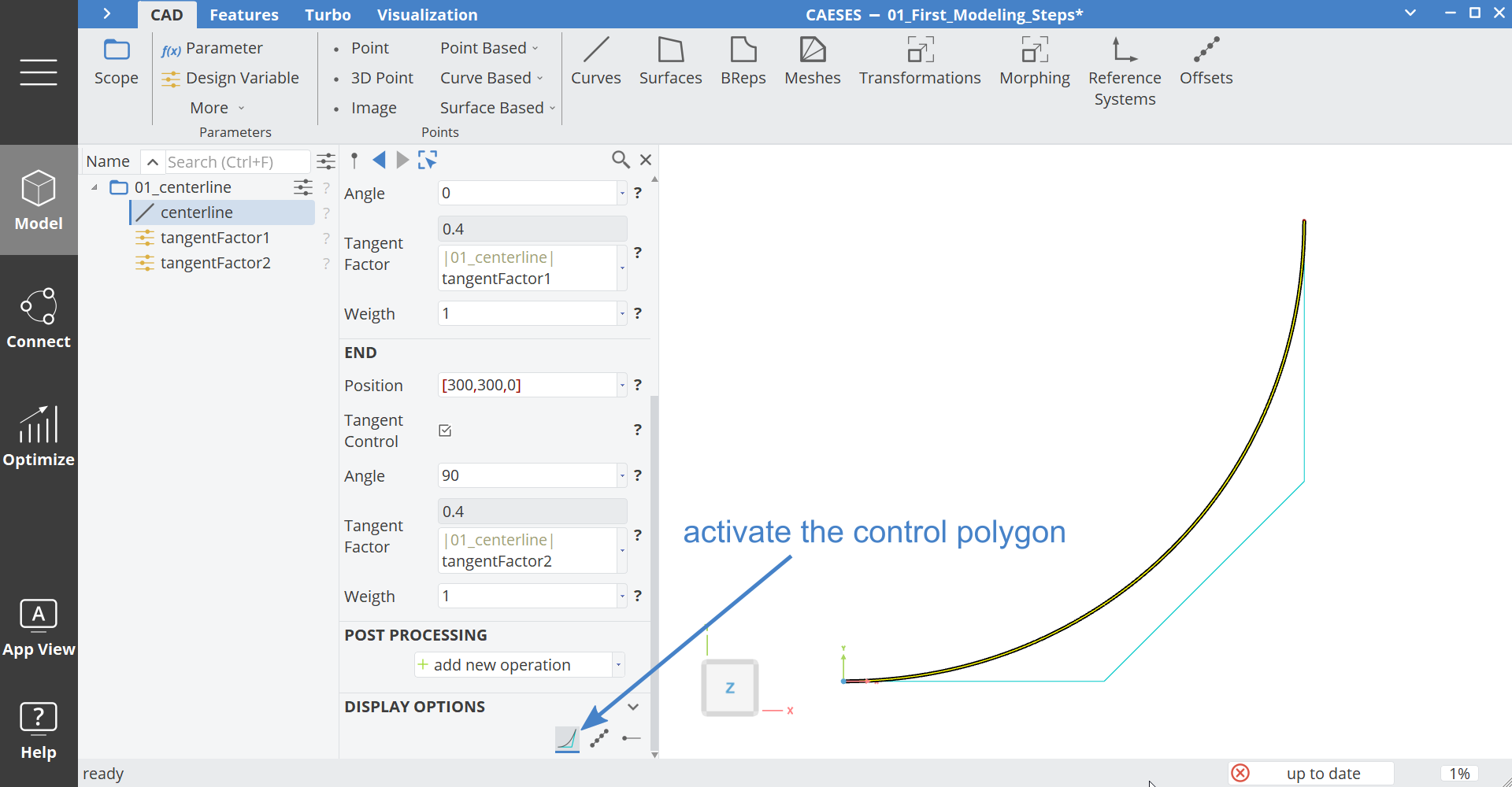
The result should look like the image below.
You can activate the control polygon of the curve in order to see the effects of the tangent factors.
Design Variable Bounds
In order to set the bounds of a design variable you can click on the edit button next to the value:
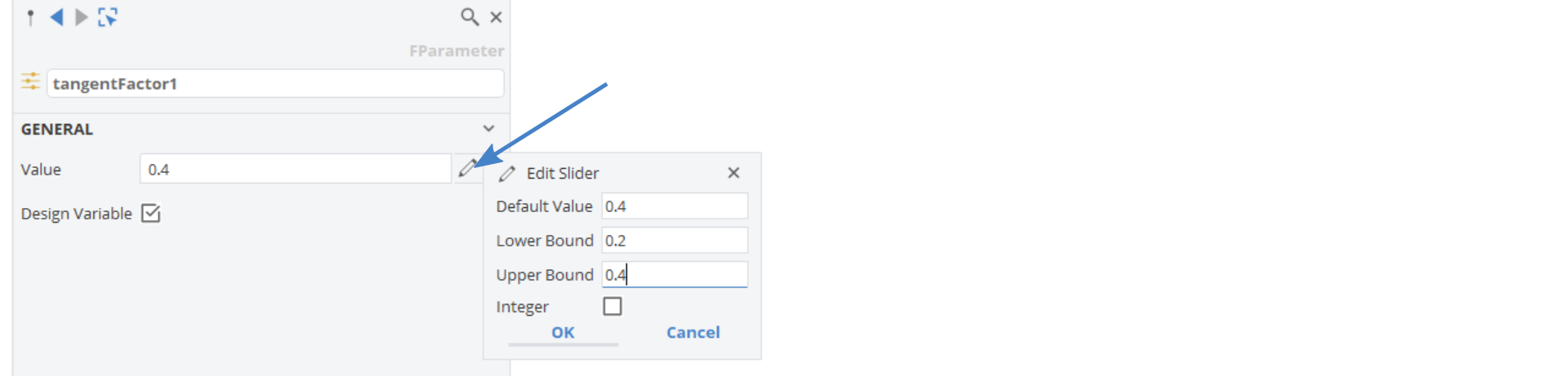
- Select tangentFactor1 and set the lower bound to 0.2 and the upper bound to
0.4. - Select tangentFactor2 and set the lower bound to 0.2 and the upper bound to
1.2.
After you have set the bounds you will get a slider in order to easily change the value. If you click on the design variable overview next to a scope, you will get an overview of all design variables inside this folder:

A parameter is used if you need expressions or links to other parameters like sqrt(9)/parameter1. A design variable can only handle a double or integer value and is used to control your model easily by hand or automatically with a design engine. You can convert a parameter to a design variable and vice versa, by activating the toggle Design Variable, however a parameter expression will be replaced by the double or integer value if you convert it into a design variable.
Profile Definition
In this tutorial we want to create a sweep surface between two different profiles. We create these profiles in this step.
Profile Start
- Click with the middle mouse button on the first scope, or somewhere else in the tree, in order to deactivate the working scope state.
- Click on the scope symbol of the first scope in order to make it invisible. The icon should then be greyed out or lighter.
- Create a Scope via Model > CAD > Scope and set the name to "02_profileStart".
- Click with the middle mouse button on this scope to make it a working scope.
Using scopes is a good way to separate and organize different components of our model.
We will create a parametric profile based on one quarter of a section, which is defined with a NURBS curve from three points. It can be controlled by radius, ellipse factor and weight.
- Create a 3D Point via Model > CAD > Points > 3D Point.
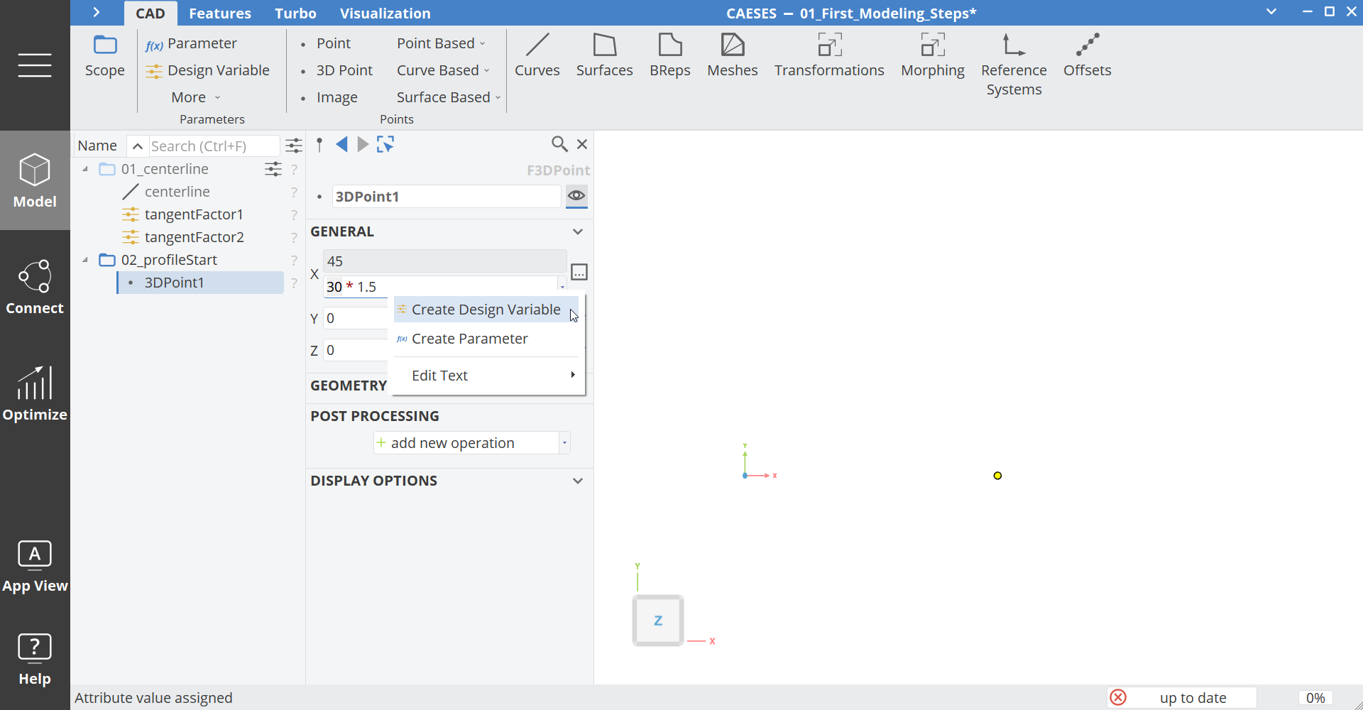
- Set the X-value to
30*1.5. - Select the
30within that expression and create a new Design Variable with a right click from it. Set the name to "radius".
-
Select the
1.5within that expression and create a new design variable with right click from it. Set the name to "ellipseFactor". -
Copy and paste the first point. The name of the second point will be "point2".
-
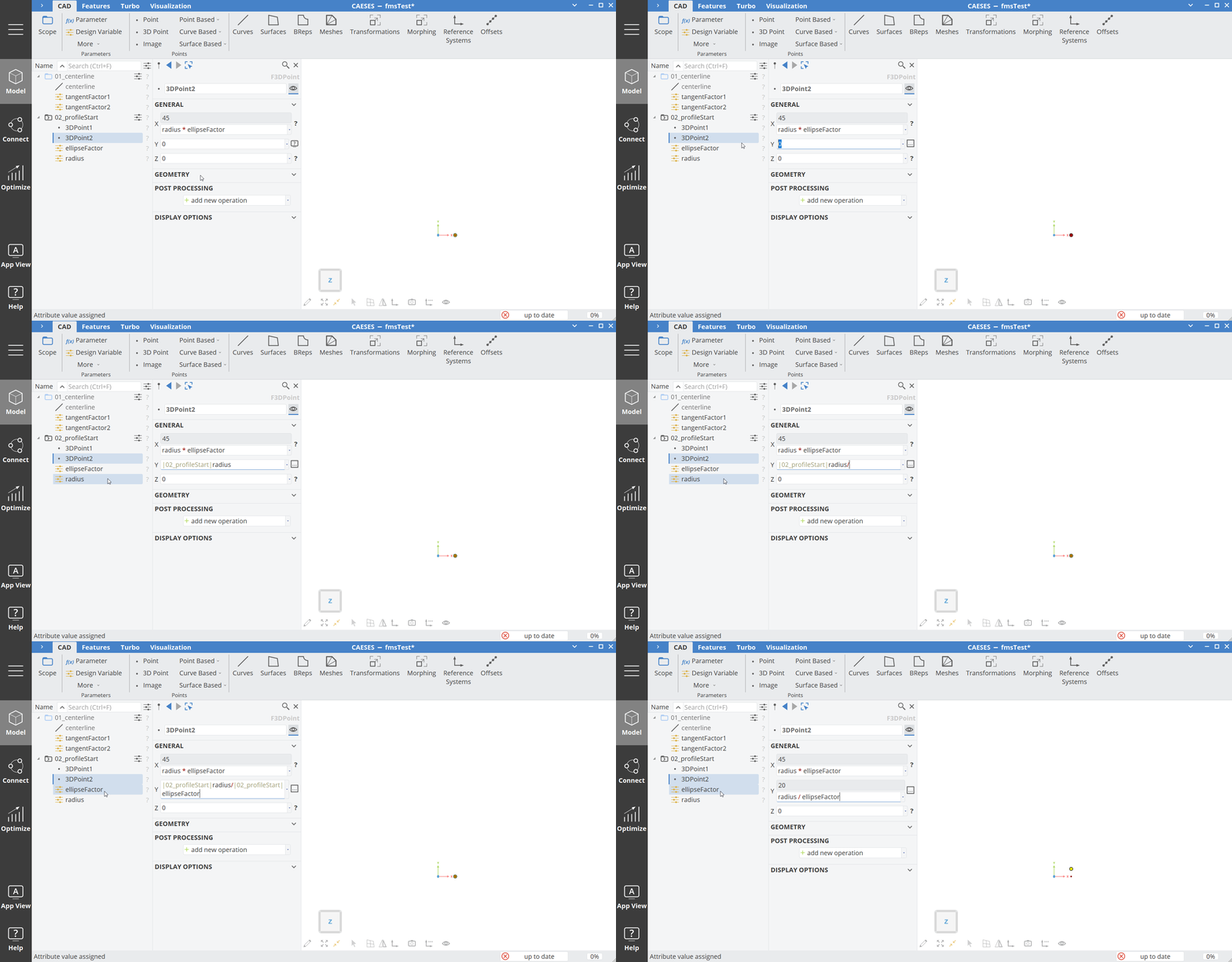
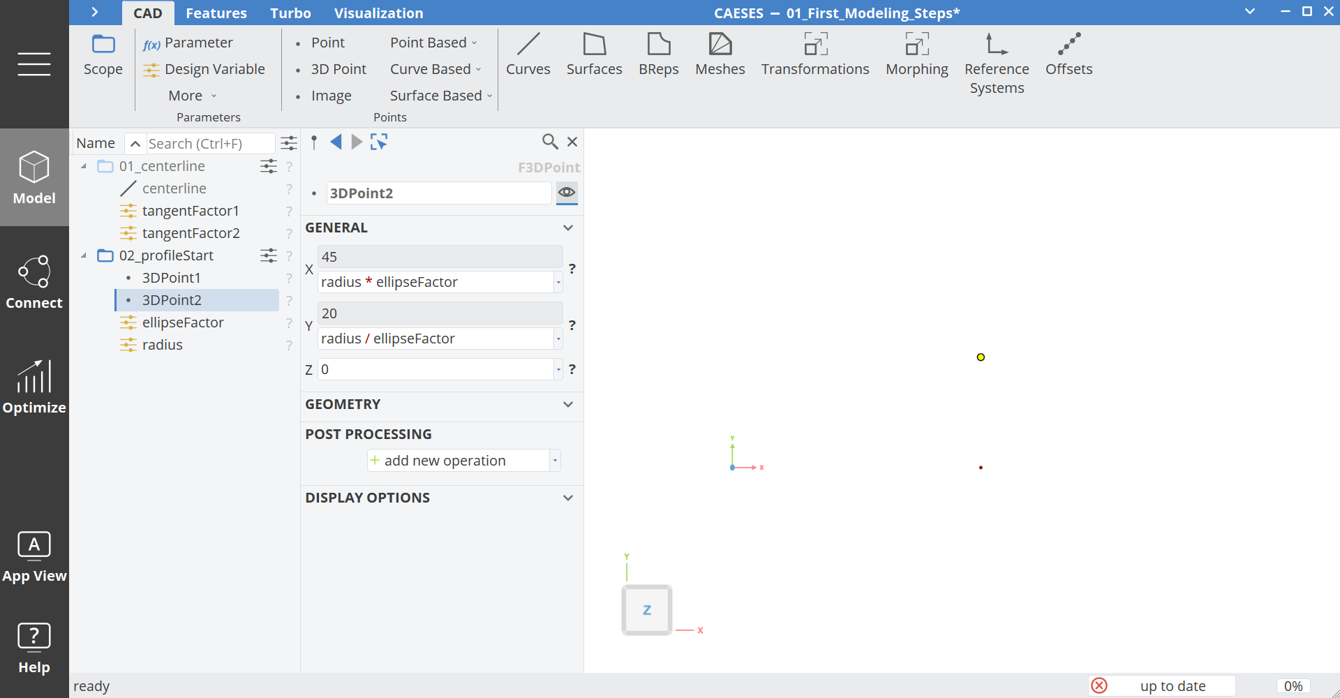
Select point2 and set the Y-value to:
radius/ellipseFactor
You can reference objects in different ways. An easy way is, to drag and drop the object to the current editor field.
However, the most common way is to select the value inside the current editor field, then press the Alt key and click the object you want to use inside the object tree or 3D window.
- Copy and paste the second point. The name of the third point will be "point3".
- Select point3 and set the X-value to
0.
Now we can create a NURBS curve from these three points.
- Select the three points starting from the first one by holding the Ctrl key.
- Create a curve via Model > CAD > Curves > Point Based > NURBS and set the name to "arc1".
In many cases it is very convenient and fast to select source objects first before you create a new object, because you then don't have to set these objects afterwards. In this case we are creating a point based curve, which needs a list of source points. When you select the source points first, they will be automatically used inside the new curve. Be careful with the order of the selection, because that order will also be used. This method is available for nearly all objects. Another simple example is the case of a ruled surface, where you would simply select two curves before you create the surface.
- Select arc1 and click on the expand icon of General.
The expand icons inside the object editor are v or ^ on the right side. They indicate that there are more options available, which are used less often.
-
Expand the General category.
-
Set the Weights vector to:
[1, sqrt(0.5)*1,1] -
Select the
1after thesqrt(0.5)*and create a design variable from it. Rename this design variable to "weightFactor".
By setting the weight of the second point to sqrt(0.5) the NURBS curve will be circular or elliptic. By multiplying that value with a factor we can change the weight easily and can always come back to a circular arc, by setting the weightFactor to 1.
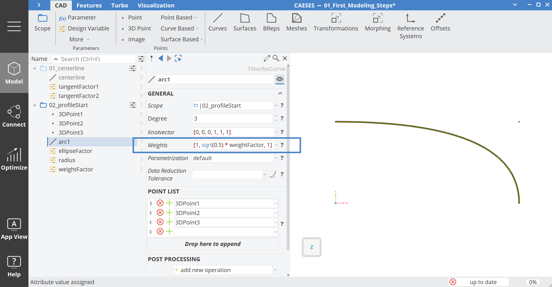
- Change the Design Variable weightFactor to
10.
Now we need to create the three remaining curves which are based on arc1.
- Select arc1.
- Create an Image Curve via Model > CAD > Curves > Curve Based > Image and set the name to "arc2".
An image curve is, as the name suggest, an image of a curve. It is mostly used for trimming operations or translations acting on an existing curve.
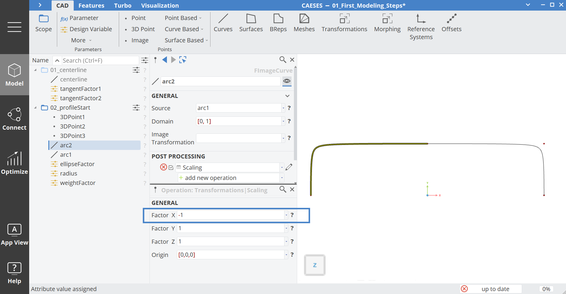
- Add a new operation via add new operation > Transformations > Scaling.
- Set the Factor X of the first scaling operation to -1 in order to mirror the curve along the X-axis.
- Copy and paste arc2. It will be automatically renamed to "arc3".
- Select arc3.
- Open the edit mode of the first scaling operation like shown below
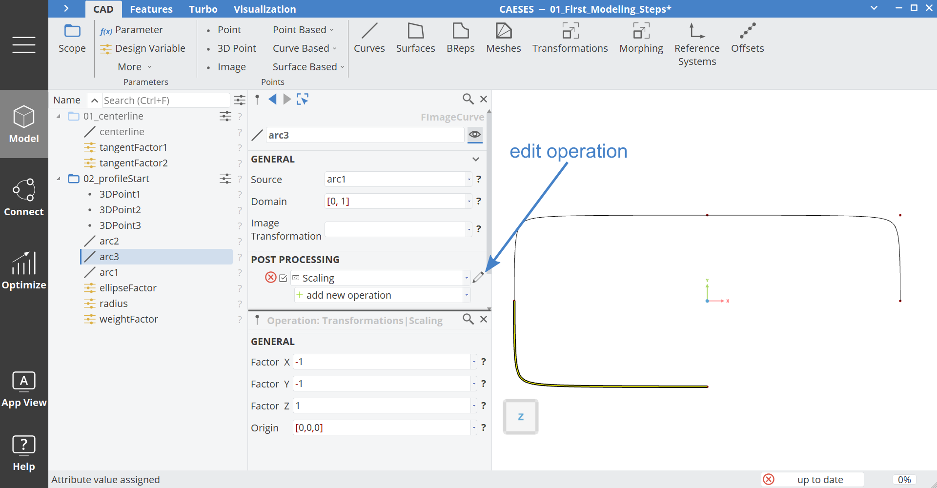
- Set the Y-value to
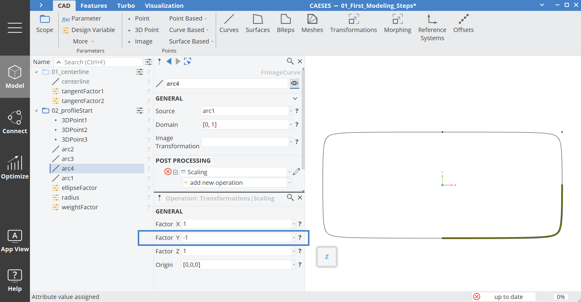
-1. - Copy and paste arc3. It will be automatically renamed to "arc4".
- Select arc4.
- Open the edit mode of the first scaling operation and set the Factor X to
1. - Make sure that the Factor Y is still
-1.
Now you should have 4 arc sections which are visually connected to each other:
In order to handle the profile as one single curve we need to combine the single curves into a Poly Curve.
- Select the 4 arcs in the correct order by holding the Ctrl key.
- Create a Poly Curve via Model > CAD > Curves > Curve Based > Poly and set the name to "profile".
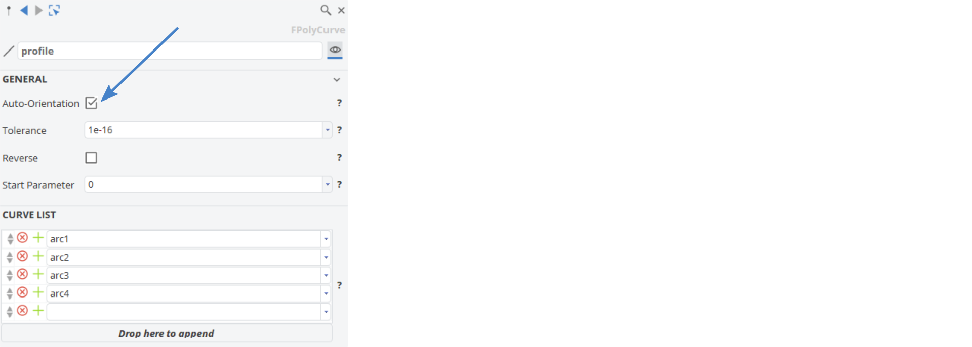
- Activate Auto-Orientation option, which is important if the orientations of the single curves are not aligned.
The Poly Curve profile can now be transformed to the needed location on the centerline.
- Select profile and add the operation add new operation > Transformations > Sweep.
- Set the Path to the curve centerline from the first scope.
Remember the Alt key selection? Click into the text editor of Path, then press the Alt key and then select with the left mouse button the centerline curve from the first scope.
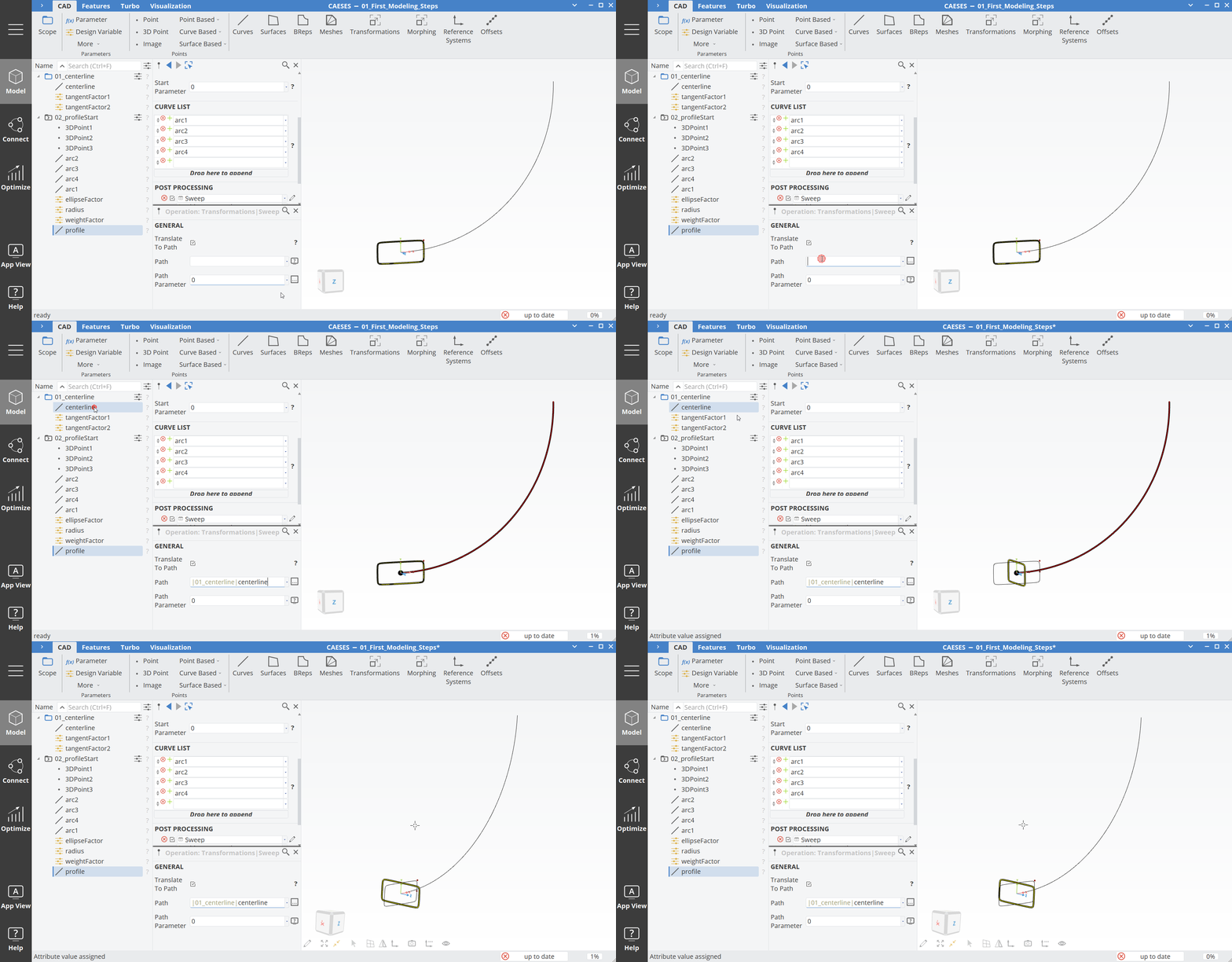
- Select the
0from the Path Parameter and create a new parameter from it. - Rename the new parameter to "sweepPos".
Design Variable Bounds
- Select the design variable radius and set the lower bound to
16and the upper bound to35. - Select the design variable ellipseFactor and set the lower bound to
0.8and the upper bound to1.7. - Select the design variable weightFactor and set the lower bound to
1and the upper bound to10.
Profile End
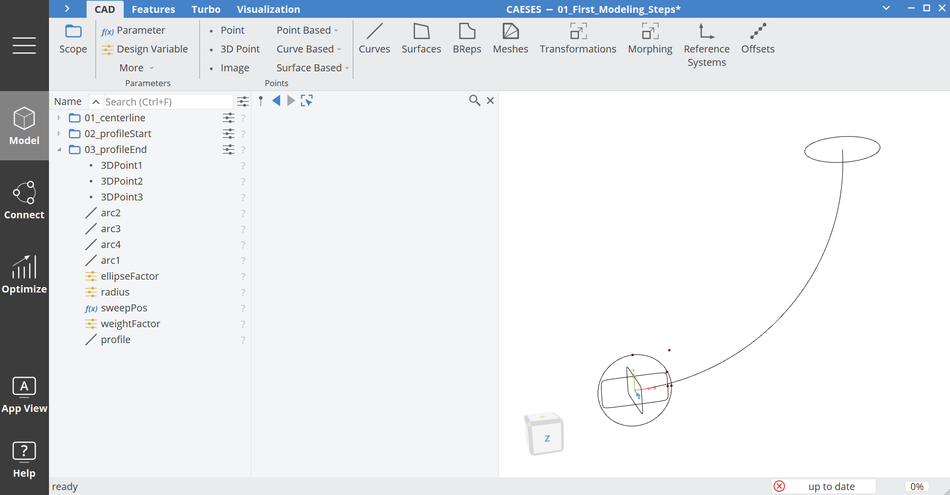
We could use the first profile to make a constant sweep surface, but in this example we want to create a sweep surface between two different profiles. Since we already have a definition of a profile, we could also use it for the end, by simply copying and pasting the scope/folder and change the values of some parameters.
- Click with the middle mouse button on the scope 02_profileStart to deactivate the working scope state.
- Copy (Ctrl+C) and paste (Ctrl+V) the scope 02_profileStart and rename it to "03_profileEnd".
- Set the parameter sweepPos to
1in order to locate the profile at the end of the centerline.
Design Variable Bounds
- Select the design variable radius and set the default value to
50, the lower bound to45and the upper bound to55. - Reset the radius value to default:

- Select the design variable ellipseFactor and set the default value to
1, the lower bound to 1 and the upper bound to1.2. - Reset the ellipseFactor value to default.
- Select the design variable weightFactor and set the default value to
1, the lower bound to1and the upper bound to5. - Reset the weightFactor value to default.
Surface and domain
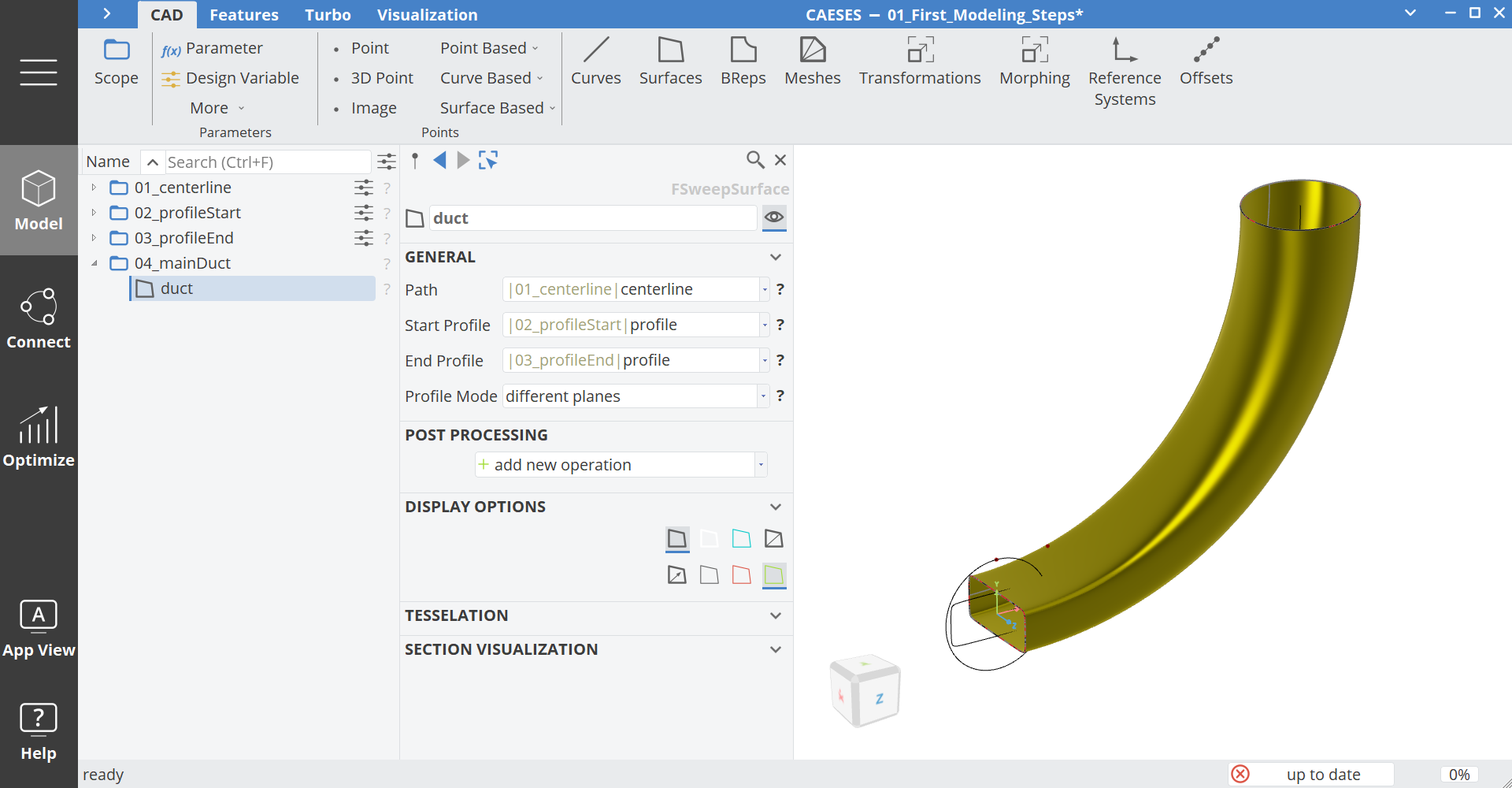
From the two profiles, we can create a sweep surface. This surface is closed afterwards at the inlet and outlet in order to create a closed fluid domain.
- Create a Scope via Model > CAD > Scope and set the name to "04_mainDuct".
- Click with the middle mouse button on this folder to make it a working scope.
- Create a Sweep Surface via Model > CAD > Surfaces > Curve Based > Sweep and set the name to "duct".
- Set the Path to the centerline curve from the first scope.
- Set the Start Profile to the profile curve from the scope 02_profileStart.
- Set the End Profile to the profile curve from the scope 03_profileEnd.
In order to create a closed domain from this surface we need to create a BRep.
- Select the surface duct.
- From the CAD ribbon create a BRep via BReps > BRep and set the name to "ductClosed".
- Hide the duct surface by clicking on the icon of duct.
An important part of the preparation of a domain, which should be used for example inside a meshing program, is the consistent naming of the different boundaries. In CAESES naming of the surfaces is done with colors. Each color has an ID which should be unique for each boundary. The ID is automatically adjusted with the RGB value. But you can also overwrite the ID. You can find the different colors in Menu > Export > Colors.
When you select ductClosed you can see that the BRep is basically created by a chain of operations. You can add, edit, move, enable, disable and delete operations. The first operation is automatically Add Sources. The Add Sources operation will stich together different surfaces or BReps. And you can group the different objects by setting a single color for this operation.
It is also important to know that a color inside a BRep is not overwritten by any other operation.
- Let's set a color for the first operation, by first clicking on the edit icon next to the operation.
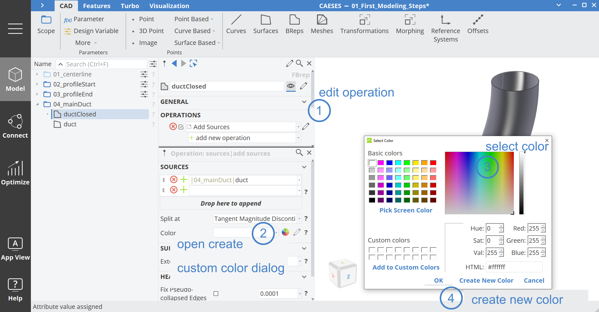
- Then click on the color wheel to create a custom color.
- A color dialog will pop up, where you can set the color value
- After you set the color value, click on Create New Color to create a new color.
- Rename the new color to "ductWall".
- Create a new operation via add new operation > Closing > Faces from Planar Curves.
- As a Source set the curve profile from scope 02_profileStart.
- Create a new color for this operation with the name "ductInlet". The method is the same as described above.
- Activate the operation by clicking on the check box left of the operation.
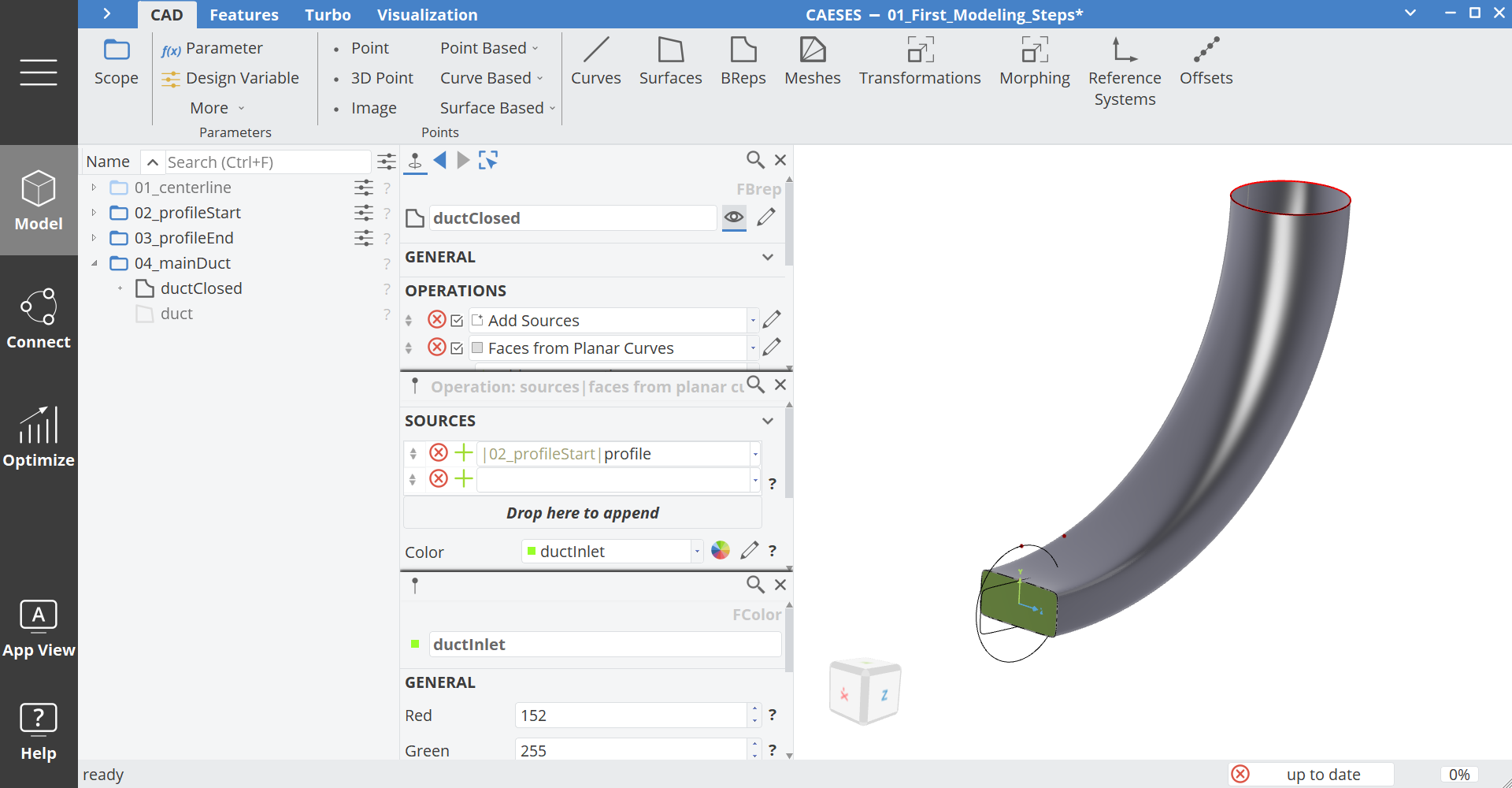
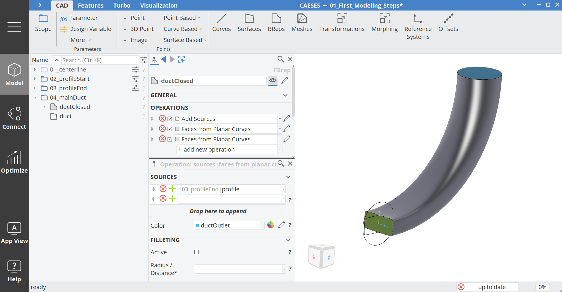
- Create a new operation via add new operation > Closing > Faces from Planar Curves.
- As a Source set the curve profile from scope 03_profileEnd.
- Create a new color for this operation with the name "ductOutlet". The method is the same as described above.
- Activate the operation by clicking on the check box left of the operation.
At the moment you can not see the colors on the BRep, because while selected it is shown in the highlight color yellow. In order to see the color, deselect the BRep with a click on any empty space in the 3D View or Object Tree.
Intake Cylinder
In this step we want to add an extra intake cylinder to the domain by using Boolean operations and fillets.
- Click with the middle mouse button on the scope 04_mainDuct to deactivate the working scope state.
- Make sure that no object is selected.
- Create a Scope via Model > CAD > Scope and set the name to "05_intakeCylinder".
- Click with the middle mouse button on this folder to make it a working scope.
- Hide the scope 04_mainDuct by clicking on the icon of the scope.
- Make 01_centerline visible if it is not already.
- Create a BRep via Model > CAD > BReps > More > Cylinder Domain and set the name to "intakeCylinder".
We want the intake cylinder be dependent on the centerline. To specify a location (3D vector) on this curve, we use the command .getpos(t). In CAESES nearly every action can be expressed with a specific command, which makes it powerful, especially when it comes to scripting. All curves are parameterized definitions and the domain of a curve is in the range [0,1], referred to as the parameter t. This makes it very simple for us to reference a location on a curve, which is relative to the length in this case.
-
Select intakeCylinder.
-
Set the Center to
|01_centerline|centerline.getPos(0.3). Follow the next steps to set the commands with auto completion correctly: -
Select [0,0,0] first, then press the Alt key and then select the centerline curve.
-
Afterwards write
.get -
Now you can press the key combination Ctrl+Space in order to get all available commands, which start with
.get.
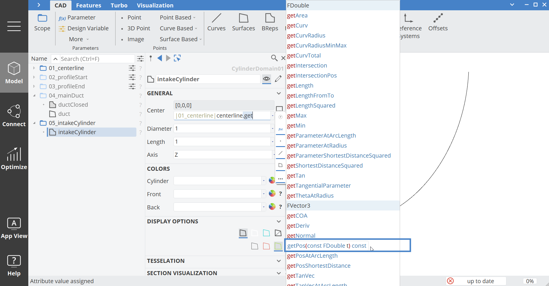
The commands are grouped by return type. We know that the return type of this command should be a vector, therefore we should look for the command in the vector group.
- Select the command
.getPos()with your mouse or with the keyboard arrows up or down.
The expression should now look like this: |01_centerline|centerline.getPos().
- Set the cursor in the parentheses of the command and press Ctrl+Space to get information about the arguments:
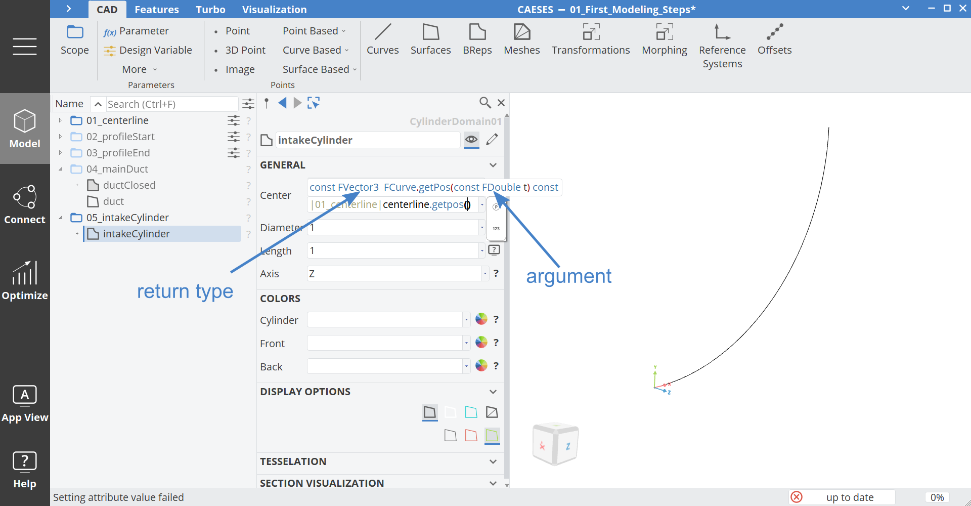
In this case we need to specify a double value, which describes the t domain of the curve.
- Write
0.3inside the brackets. - Select the
0.3and create a design variable from it. - Rename the design variable to "intakePos".
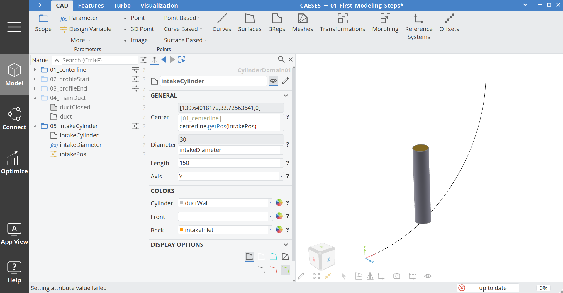
- Set the Diameter to
30and create a new Parameter from it. Rename it to "intakeDiameter". In this case we use a Parameter instead of a Design Variable, because we do not want to change the value automatically inside a design engine. - Set the Length to
150. - Set the Axis to Y.
- Set the color of Cylinder to ductWall.
- Create a new color for the Back face by clicking on the color wheel next to the combo box. Rename the color to "intakeInlet".
Design Variable Bounds
- Select the design variable intakePos and set the lower bound to
0.2and the upper bound to0.4.
Combining Objects to One Domain
In this final step we want to combine the two separate domains into one domain and add a fillet at the junction.
- Click with the middle mouse button on the scope 05_intakeCylinder to deactivate the working scope state.
- Make sure that no object is selected.
- Create a Scope via Model > CAD > Scope and set the name to "06_finalDomain".
- Click with the middle mouse button on this folder to make it a working scope.
- Select the BRep ductClosed from 04_mainDuct.
- Create a BRep via Model > CAD > BReps > BRep and set the name to "finalDomain".
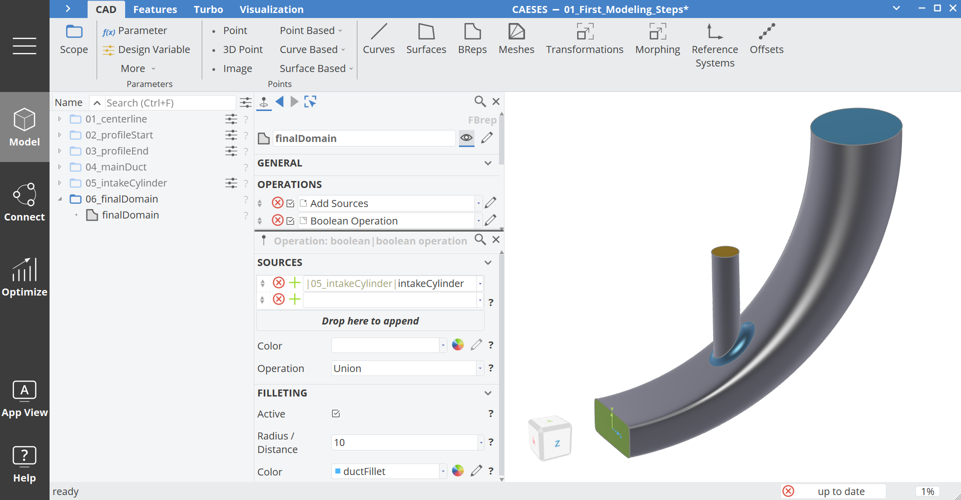
- Create a new operation add new operation > Boolean > Boolean Operation.
- Set the Source to the BRep intakeCylinder from scope 05_intakeCylinder.
- Activate the fillet option.
- Set the Radius / Distance to
10. - Expand the editor of Filleting and create a new color for the fillet with the name "ductFillet".
- Activate the Boolean Operation.
When you hide all scopes (click on the scope icon to hide all objects inside the scope) except the last one, you can have a clean view on the final BRep.
CAESES Project File
If you want to take a look at the finalized model you can find the resulting CAESES project file first-modeling-steps.cdb here: