Meta Surface Creation
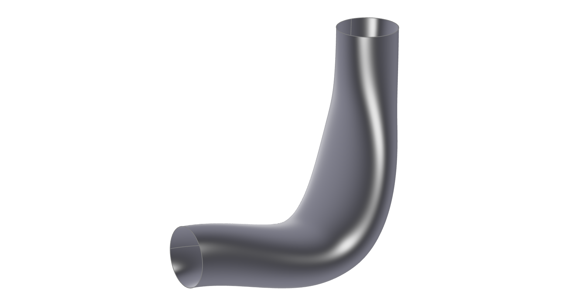
Curved Duct with Meta Surface
As a specialized CAD solution, CAESES provides a set of different surface types in order to create flexible parametric geometry models. The meta surface is a bit distinct, when you compare it to common surface types in other CAD systems. Basically, a meta surface is a parametric sweep surface with more user controls and hence a higher flexibility, especially in the context of efficient shape optimization with simulation tools. It allows you to massively reduce the total number of parameters, while always generating smooth and feasible surface shapes. In particular, meta surfaces are ideal for complex free-form surfaces such as ducts, wings, exhaust ports, volutes, blades, ship hulls etc., to foster innovation with more customized and ready-to-automate CAD models.
In the first tutorial First Modeling Steps we created a sweep duct surface which blends the sections at start and end linearly. Now we want to get more detailed control of the parameters within the sweep. Therefore we will use the Meta Surface.
Basic Concept
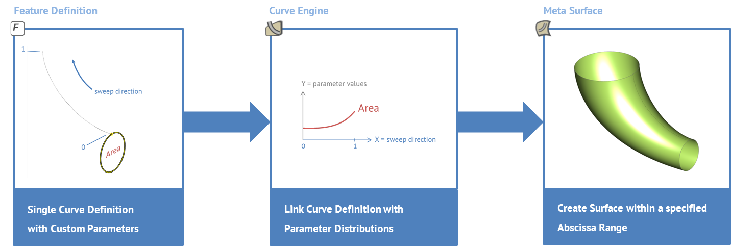
You can find more general information of Meta Surfaces here. In short, a Meta Surface is created with the following steps:
-
In the first step, you create a feature definition which describes your curve (that you want to sweep). This curve has a set of parameters including the "sweep parameter" that will be used to sweep the curve into the 3D space and to create the surface.
-
Secondly, you create function graphs for all of your curve parameters. Most often, this is done in the XY-plane, where normalized functions are define, i.e., running in the x-interval
[0,1]and in the y-interval[0,1]. The sweep parameter of your definition typically has a linear function, e.g. if it is a curve path parameter there would be a linear function from0to1.
The use of functions reduces the number of free variables drastically, and typically creates smooth surface shapes if you use smooth functions.
-
As an intermediate step now, create a curve engine (Model > CAD > Surfaces > Meta Surface > Curve Engine) which connects the curve definition to the parameter functions. This engine is now able to create your curve at any 3D location according to your function graphs.
-
In the last step you create a meta surface that takes the curve engine and generates the surface.
The following picture illustrates the whole process:
Model Preparation
We start by opening the project file from the First Modeling Steps tutorial
Get Started- Save your project via Menu > File > Save Project As.
- Delete the scopes 03_profileEnd to 06_finalDomain. After that we should just have to two scopes 01_centerline and 02_profileStart.
- Make both scopes 01_centerline and 02_profileStart visible with a click on the scope icon.
Feature Definition
As already described, we need the profile definition in form of a script. This script is called Feature Definition in CAESES. We can write the Feature Definition from scratch, or we can create the Feature Definition based on the geometry we already have created in the GUI. For this tutorial we use the second option, since this is easier.
A Feature Definition is a little script or program, which creates some output geometry with the help of some input arguments. In this specific case, we want to create a profile on a centerline. The profile curve is the output of the Feature Definition. In order to create the output, we need some input arguments. These are in this case the parameters for the shape of the profile like ellipseFactor, radius, ... but also the curve centerline, since this information is needed to align the profile.
We create a Feature Definition from the selected geometry. All objects which are needed to create the selected objects and which are not selected will be used as input arguments of the Feature Definition.
Let's start:
- Select all objects in the scope 02_profileStart but not the Parameters and Design Variables
- Right click and select Create Feature Definition.

A new dialog will pop up, with the settings of the Feature Definition. Let's go through the different tabs and do some simple modifications.
General
- Select the General tab
- Set the Type Name of the Feature Definition to "profileDefinition"

Arguments
- Select the Arguments tab.
The input arguments are shown in a table view with settings in each column.
Type: The object type of argument. The most common one is a double type (decimal number), but as we can see in our example, we can also have all other geometry types as input arguments like the FCurve.
Name: Argument name as it is used in the feature code in Create Function
Category: You can group certain arguments in order to get a structured interface.
Label: Name of the argument as shown in the interface
- Change the category name of the three first double types to "Shape"
- The centerline and sweepPos do not have a category name thus will be shown in the General category of the feature interface.

Create Function
- Select the Create Function tab.
Here you will find the actual code of the Feature Definition, containing the Command form of all steps we took in the User Interface. We don't have to do anything here for now.

Attributes
- Select the Attributes tab.
This tab defines which objects inside the feature are accessible from outside the feature. You can also define the Type Provider of the feature.
-
Activate the Type Provider toggle at the profile curve. This means that this Feature Definition can be handled like a curve within the project.
-
Press on Apply to apply any changes to the Feature Definition.

-
You can close now the dialog of the Feature Definition.
-
You will find all Feature Definitions of the project in Model > Features
-
Right click on profileDefinition and select Create Feature.

- Switch back to the Model > CAD tab.
- Right click on scope 02_profileStart and select delete.
- Select the instance of the Feature Definition profileDefinition1
- Set the centerline from the first scope as the input argument of the feature:

- Play with the sweepPos and Shape input argument.
- Delete the feature instance profileDefinition1, since this was just created for testing the Feature Definition.
Parameter Functions
Now we can prepare the parameter functions, which describe the parameter value at each sweep position.
- Create a scope via Model > CAD > Scope and set the name to "functions".
- While functions is selected, create another scope via Model > CAD > Scope and set the name to "02_duct".
- Make the scope functions your working scope with a click of the middle mouse button.
- Open the 3D Overview window by clicking with the right mouse button on the ribbon and selecting 3DOverView.
- In the 3D Overview window activate the filters with a click on the eye button in the bottom action bar.
- Inside the filter toolbar, click on the Search button and set the name filter to "functions". This will just show all objects which are located in the scope functions.

- Create a 2D Diagram via Model > Visualization > 2D Diagram.
- Set the Name X Axis to "sweep position".
- Set the Name Y Axis to "parameter value".
- Deactivate the title.
Now let's create some interpolation curves, which are based on three points. We can scale the Y-coordinate of the curves in order to have all functions visible in one view.
- Create a 3D Point via Model > CAD > Points > 3D Point.
- Set the Y-coordinate to
0.45and leave the X-coordinate as0. At a later stage we will scale the function by 100. - Deselect everything and create another 3D Point via Model > CAD > Points > 3D Point.
- Set the X-coordinate to
0.5. - Select the
0.5, right click on it and create a Design Variable from it. Set the name to "radiusPositionMid". - Set the Y-coordinate to
50/100. - Select the
50, right click on it and create a Design Variable from it. Set the name to "radiusMid".

- Deselect everything and create another 3D Point via Model > CAD > Points > 3D Point.
- Set the X-coordinate to
1. - Set the Y-coordinate to
0.45.
From these three points we can create an Interpolation Curve.
- Select the three points 3DPoint1 to 3DPoint3.
- Create an Interpolation Curve via Model > CAD > Curves > Point Based > Interpolation.
- Rename the curve to "radiusFunction".
In order to have a smooth connection to start and end profile, we can set the tangents to zero.
- Select radiusFunction.
- Select 3DPoint1 in the point list and press the open squared bracket
[. This will enclose the hole selection with squared brackets. - Inside the brackets write
[3DPoint1,0]in order to set the tangent at the first point to zero:

- Do this also for the last point.
- Now select the three points, the curve and the two Design Variables.
- Create a scope via Model > CAD > Scope and set the name to "radius".
- Copy and paste the scope radius.
- Select the new scope radius01 and set the name to "ellipseFactor".
- Inside this scope rename the Design Variable radiusMid to "ellipseFactorMid" and set the value to
1.2. - Inside scope ellipseFactor select the Design Variable radiusPositionMid and rename it to "ellipseFactorPositionMid".
- Inside scope ellipseFactor select the curve radiusFunction and rename it to "ellipseFactorFunction".
- Inside scope ellipseFactor select the 3D Point 3DPoint1 and set the Y-coordinate to
1. - Inside scope ellipseFactor select the 3D Point 3DPoint2 and set the Y-coordinate to ellipseFactorMid.
- Inside scope ellipseFactor select the 3D Point 3DPoint3 and set the Y-coordinate to
1.

Now we need a linear function for the sweep position.
- Create an Line via Model > CAD > Curves > Line.
- Set the name to "sweepPosFunction".
- The default values of the Line are fine.
Curve Engine
At this point we can continue by setting up the curve engine.
- Click with the middle mouse button on the scope 02_duct in order to make it the current working scope.
- Create a Curve Engine via Model > CAD > Surfaces > Meta Surface > Curve Engine.
- In the argument Definition select our Feature Definition profileDefinition.
- Click somewhere in the Object Editor to let the Curve Engine update itself. You should see the fields corresponding to the Input Arguments of the Feature Definition appear.
- In the argument Base Curve select the curve profile.
- For the argument Centerline choose the centerline curve from the first scope 01_centerline.
- For the argument SweepPos choose the line sweepPosFunction.
- For the argument Radius choose the curve radiusFunction.
- You can see the
1in squared brackets behind the curve. This is the Y-scaling. Set the value to100. - For the argument EllipseFactor choose the curve ellipseFactorFunction.
- Set the argument WeightFactor to
1.
The inputs of the curve engine are shown below:

Meta Surface
In this final steps we can create the Meta Surface from the curve engine. The Meta Surface gets the parametric profile at each position from the Curve Engine and connects them using a Lofted Surface.
- Select the curveEngine1.
- Create a Meta Surface via Model > CAD > Surfaces > Meta Surface > Meta Surface.
- Set the name to ductSurface

The representation type is by default Skinning, which will keep the parametrization of the underlying profile curves from the Feature Definition.
The number of Interpolated Points in Surface Direction means, how many sections are used along the parametric sweep. In this example 15 is enough, but if you have more complicated shapes, you may want to increase this number.
Design Variable Bounds
Finally we can set the bounds of the Design Variables, in order to easily modify the shape.
- Click on the Design Variable overview next to the scope 02_duct.
- Click on the Edit button of the first row.
- Click on the Edit button of the individual Design Variable, in order to set the bounds:

- Click on the Edit button of ellipseFactorMid and set the lower bound to
0.8and the upper bound to1.5. - Click on the Edit button of ellipseFactorPositionMid and set the lower bound to
0.4and the upper bound to0.6. - Click on the Edit button of radiusMid and set the lower bound to
45and the upper bound to60. - Click on the Edit button of radiusPositionMid and set the lower bound to
0.4and the upper bound to0.6.
Now you can play with the shape and also try to create some variants with the help of a Sobol algorithm as described in the tutorial Geometry Variation and Assessment.

CAESES Project File
If you want to take a look at the finalized model you can find the resulting CAESES project file meta-surface-duct.cdb here: