Advanced Propeller Workflow

PropellerThis functionality requires the Propeller add-on to be enabled. 5.3.0This functionality requires CAESES version 5.3.0 or later.

In this tutorial, we will create a parametric propeller model from start to finish using the propeller workflow in CAESES. The tutorial covers the generation of a conventional propeller design, with the flexibility to create unconventional variants such as tip rake and highly skewed propellers.

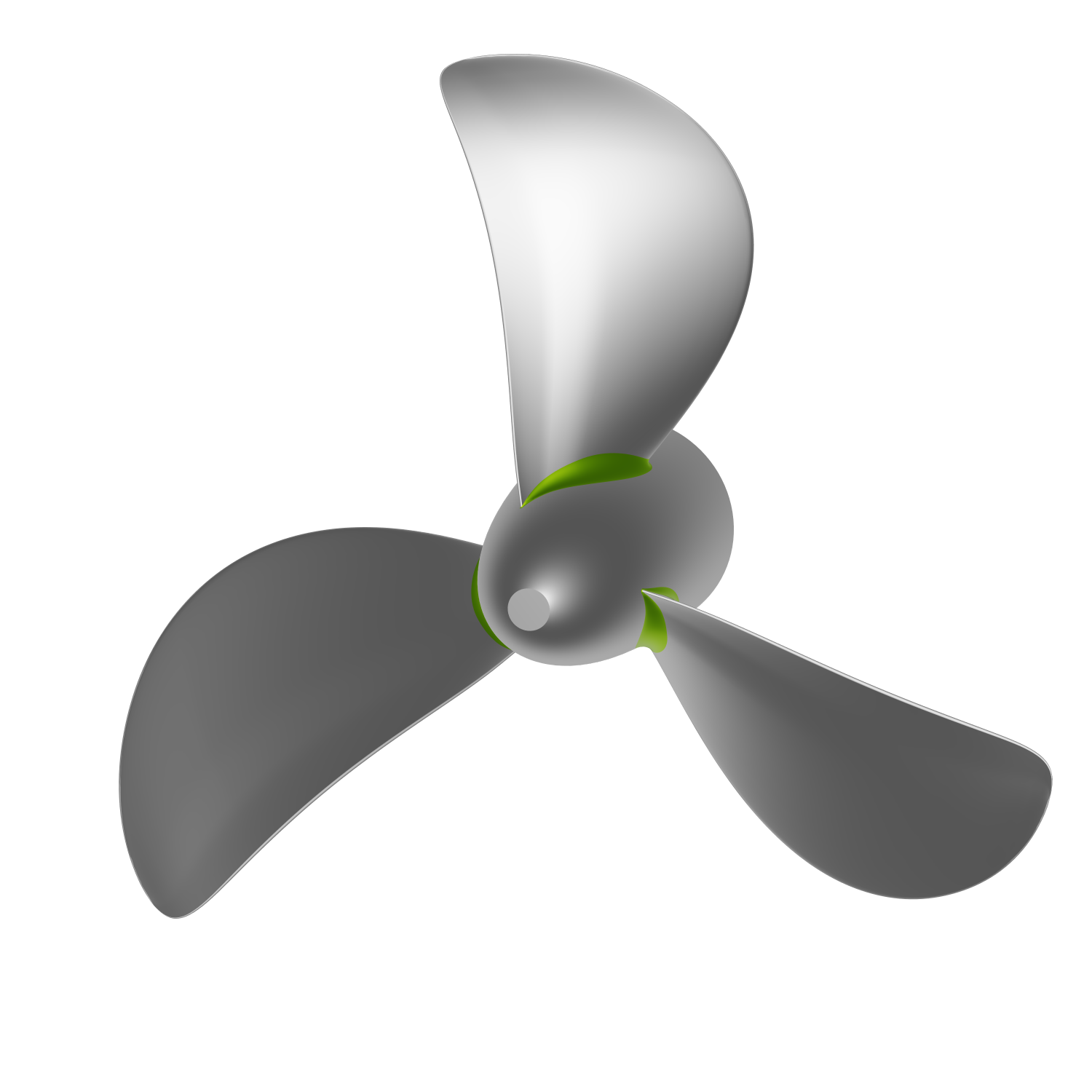
This project starts from scratch and follows the propeller workflow, which enhances propeller design in CAESES. The propeller workflow provides a step-by-step guide through the geometrical modeling process of a fully-parametric propeller design. It empowers users to boost their productivity by providing a structured workflow, making it easy to parameterize a propeller, as demonstrated in this tutorial.

Additionally, another goal of this tutorial is to familiarize you with the propeller workflow so that you feel comfortable experimenting with and changing its settings. Before proceeding further, it is recommended to review the General Overview of the Propeller Workflow.

set project units

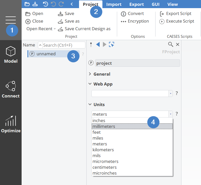
Before starting this tutorial, set the Project Units to millimeters.

To start, navigate to the Model workspace > Propeller tab > Workflows category > *Propeller > Advanced Propeller Workflow in the Propeller tab of CAESES.

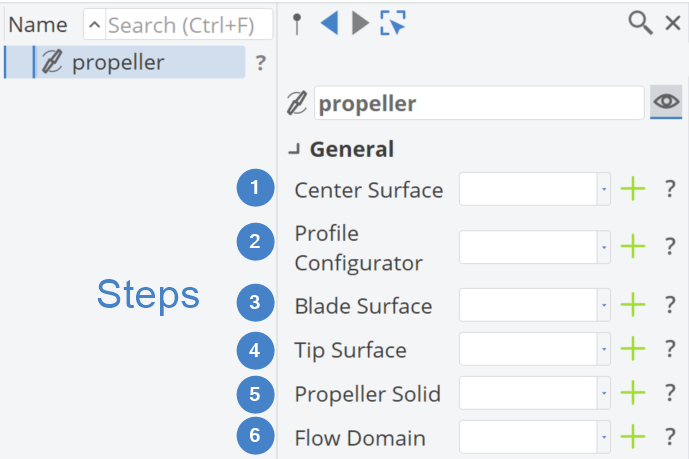
Once clicked, you should see the layout below, providing an overview of the project structure and this tutorial. Simply follow the step-by-step process by clicking the green plus buttons as you go.

Animations in this Tutorial

Throughout this tutorial, various animations illustrate the impact of different Design Variables on the final propeller geometry. If some visualizations appear more advanced than the current step, don’t worry, you’ll be guided to that point soon!

Center Surface

The first step in the propeller design workflow is defining the Center Surface.

• Click the plus button next to Center Surface.

This creates a center surface that incorporates information from various radial distributions, which are typical in propeller design. The workflow will create these functions that we will customize in this section. To do so, for each distribution, you will have to:

• Click the plus button to create a 3rd-degree B-Spline Curve.
• Select the corresponding number of control points given in the title

info

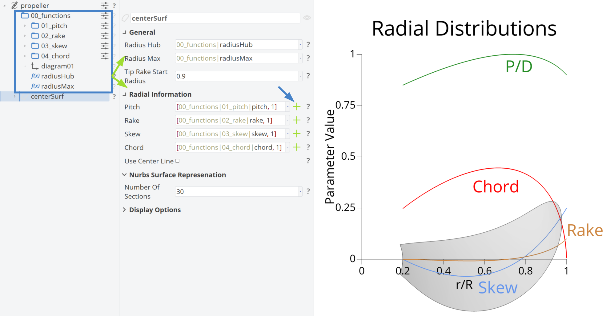
The scope structure for radial distributions follows the naming convention 0x_functionName for Center Surface. Design variables impacting each distribution are organized within their respective scopes.

Pitch Function with 3 Points

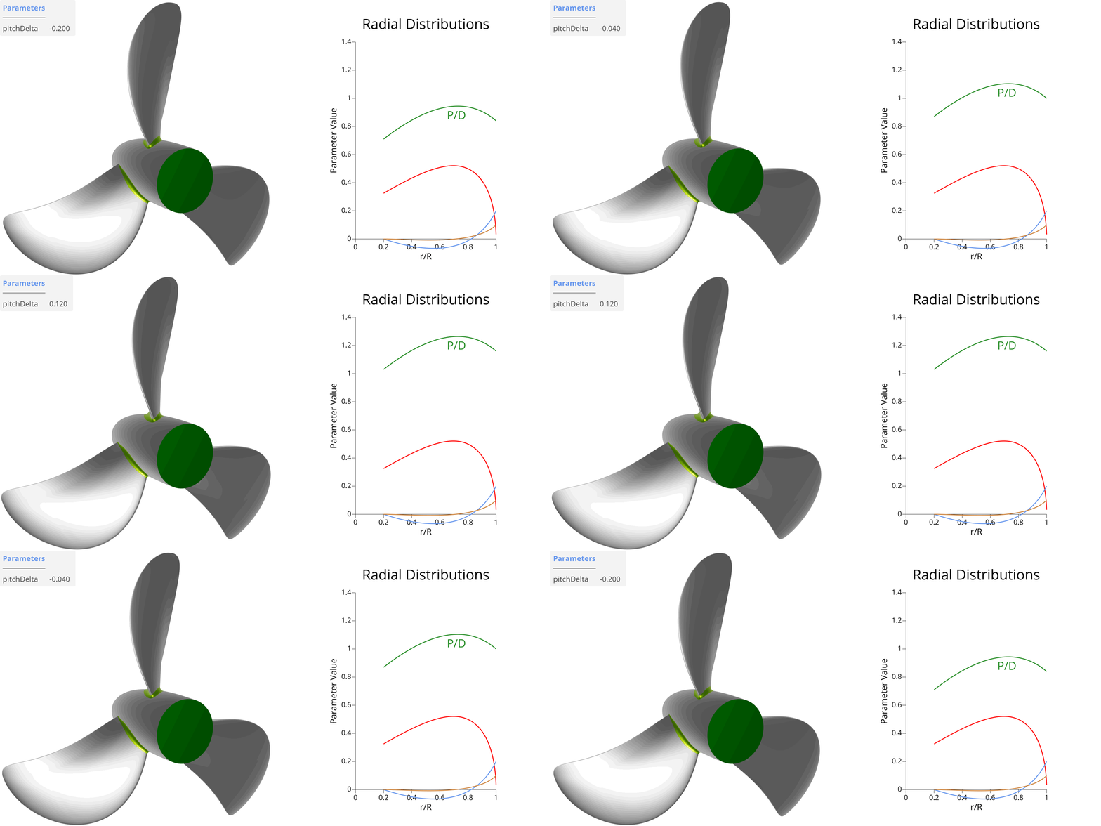
The Pitch function is normalized to the diameter (P/D). This function is controlled by a single design variable named pitchDelta, which shifts the entire function up or down while maintaining its shape.

• Set the range of pitchDelta to -0.2 to 0.2, with a default value of 0.0.
• pitchRoot and pitchTip should be set to 0.9 and 1.0, respectively.
  • Pitch at the root and tip is decreased compared to values at 0.7 r/R.

In the animation below, you can see the effect of the pitchDelta parameter on the propeller model.

Rake Function with 4 Points

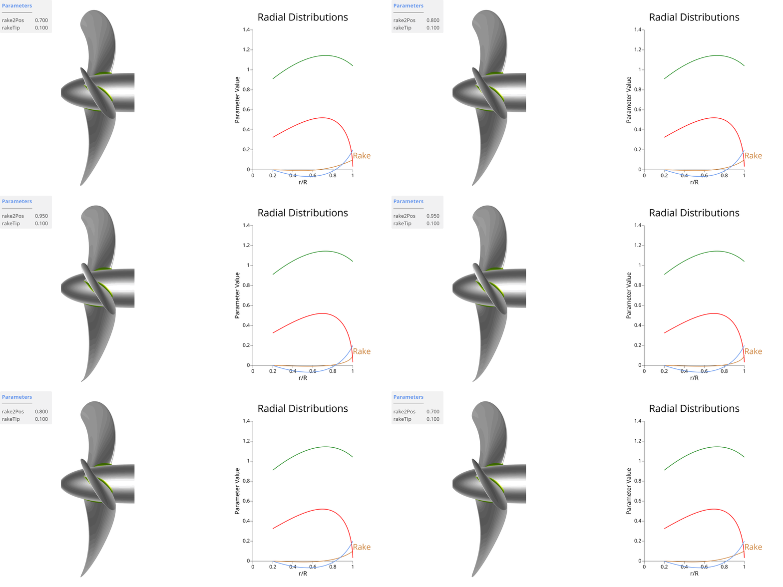
The Rake function is controlled by two design variables:

• Set the range of rake2Pos from 0.7 to 1.0, with a default value of 0.85.

  • Adjusts the shape of the Rake function:
    • 0.7 indicates a linear behavior.
    • 0.85 results in a more curved shape.
    • 1.0 leads to a tip-rake design.

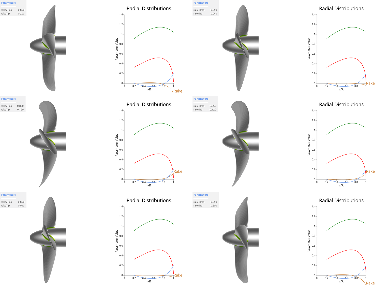
• Set the range of rakeTip from -0.2 to 0.2, with a default value of 0.1.

  • Controls the magnitude of the rake:
    • Negative values indicate forward rake.
    • Positive values indicate backward rake.

In the animations below, you can see the effect of the rakePos and rakeTip parameters on the propeller model.

Skew Function with 3 Points

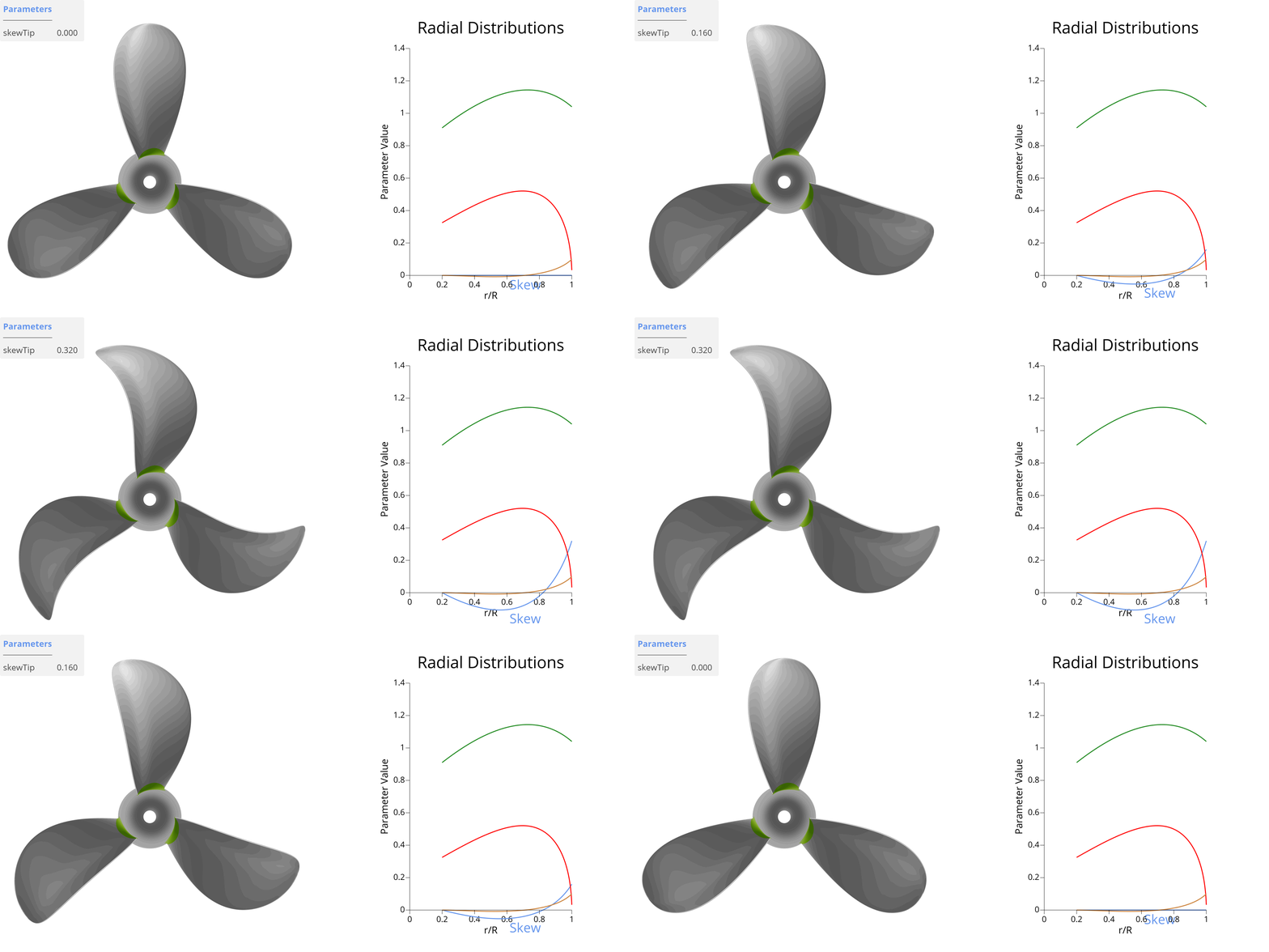
The Skew function is controlled by a single design variable named skewTip, which represents the Y value at the tip of the blade.

• Set the range of skewTip from 0 to 0.4, with a default value of 0.2.
  • This allows for designs ranging from non-skewed to highly skewed propellers.

In the animation below, you can see the effect of the skewTip parameter on the propeller model.

Chord Function with 5 Points

The Chord function is controlled by a single design variable named chordMax, which represents the Y value of the middle control point of the function.

• Set the range of chordMax from 0.6 to 0.7, with a default value of 0.65.
  • It shifts the point in the Y-direction and adjusts the position of the other control points accordingly.

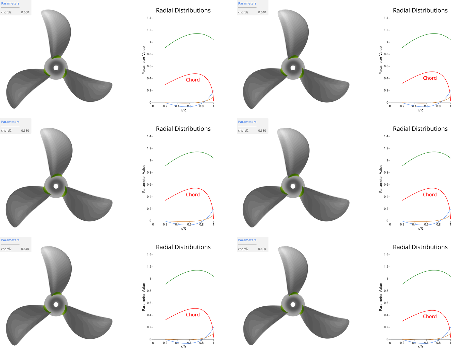
In the animation below, you can see the effect of the chordMax parameter on the propeller model.

Final 2D Radial Distributions

In the figure below, the radial distributions, we created in the previous steps, are illustrated for the creation of the central center surface, starting at radiusHub = 0.2 and ending at radiusMax = 1.

tip

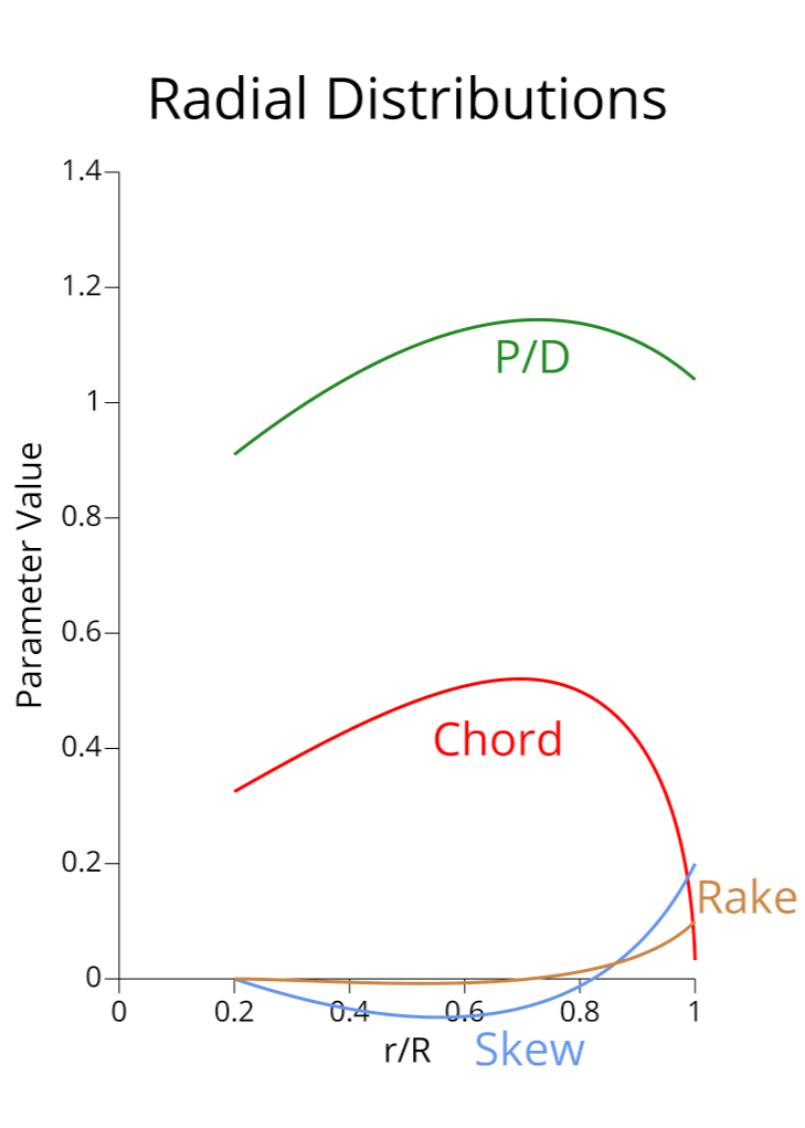
All remaining Design Variables used in the 2D Radial Distributions that are not mentioned above can be converted to Parameters by unchecking the box Design Variable.

Profile Configurator

For this tutorial, a NACA 66 mod a=0.8 airfoil is used, specifically designed for marine propeller applications.

Camberline: The parameter a = 0.8 indicates that the airfoil provides constant lift over the first 80% of the chord, with a linear decrease to zero at the trailing edge, shaping the camberline. This design helps to reduce cavitation and improves the propeller performance.

Thickness curve: The modification (mod) involves thickening the edge regions of the NACA 66 section, adjusting the thickness curve to better withstand mechanical stress. The original thin edges of NACA 66 sections were prone to damage in marine environments, making this adjustment particularly beneficial.

• To apply this, click the plus button in the propeller component GUI for the Profile Configurator and select the option: Profile Configurator via Camberline and Thickness.
• Next, for the Camberline, click the plus button and choose NACA a=0.8 Modified.
• For the Thickness curve, select Thickness Distribution for NACA 66.
• With the camberline and thickness curves, you can generate the Profile Curve by clicking on the green plus button.
• Click the Create Definition play button to create the Profile Definition, which is needed for the final blade surface creation.

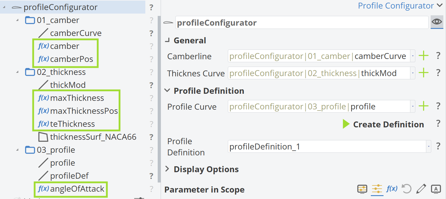
Now, the Profile Configurator GUI should look like this:

Modifying Leading Edge & Trailing Edge Thickness

Further modifications can be applied to the Thickness Curve (called thickMod in the scope thickness), especially in regions of interest such as the Leading Edge (LE) and the Trailing Edge (TE) of the Profile.

tip

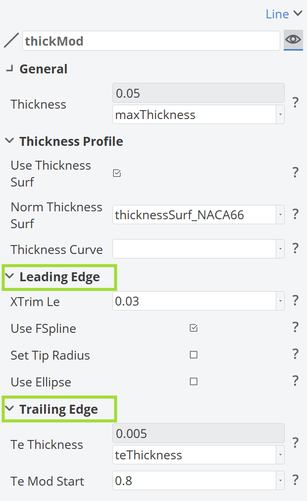
• Leading Edge: You may change the XTrim Le to modify the leading edge. Additionally, you can also check the boxes Set Tip Radius or Use Ellipse.
• Trailing Edge: You may modify the value of the teThickness parameter or set a different value at Te Mode Start.

Blade Surface

In the propeller component GUI, continue to

• click the plus button for the Blade Surface,
• select the newly created blade component in the object tree, and
• then click on Blade Surface again.

This will create three objects blade (type FPropellerBlade), tipGap (type FParameter), bladePrepared (type FImageSurface).

By selecting the blade surface (type FPropellerBlade), you can add distributions for the following functions in the Profile Parameter section by clicking on the plus button. For each function, you may choose Distribution via B-Spline Curve. All functions get created in the scope named "functions" in the blade component.

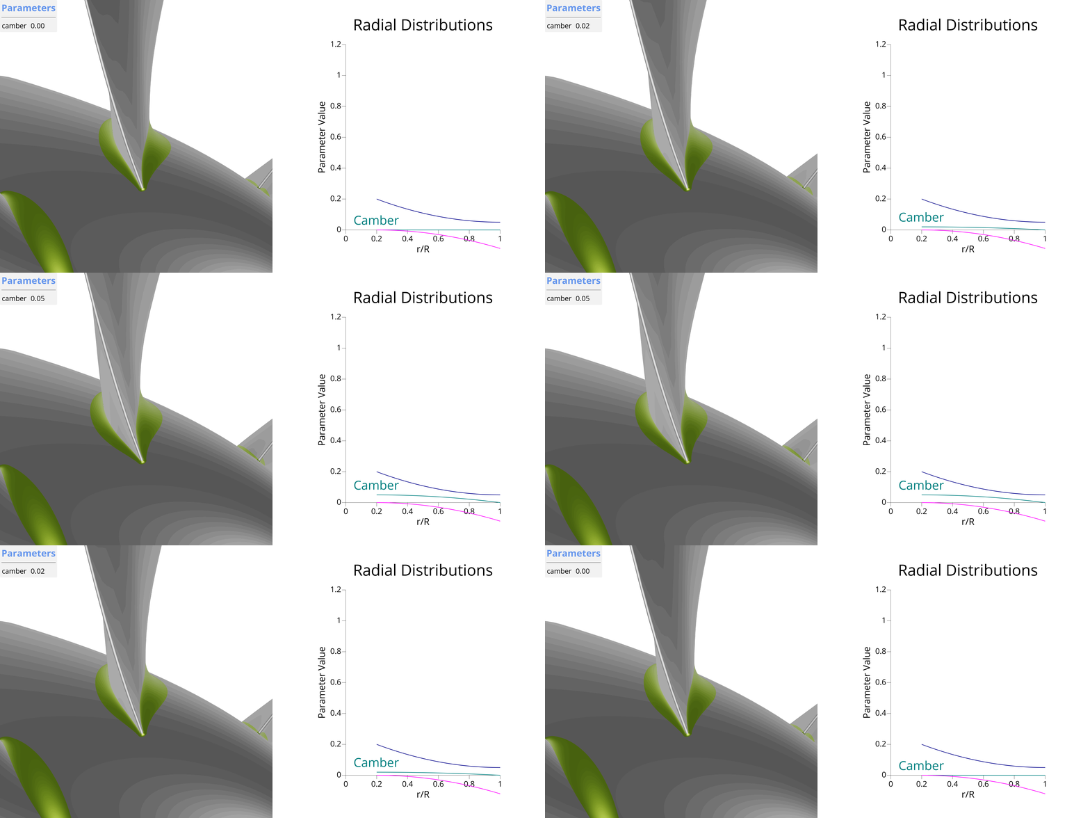
Camber

The Camber distribution describes the maximum camber of each profile in the chordwise direction. This function is controlled by a single design variable named camber_00.

• Set the range of camber_00 from 0.00 to 0.06, with a default value of 0.03.
• Convert camber_01 and camber_02 to parameters and set them to 0.
  • This is designed to achieve the greatest camber in the spanwise direction at the root of the blade, gradually decreasing towards the tip and reaching zero camber at the tip.

In the animation below, you can see the effect of the camber_00 parameter on the propeller model.

Maximum Thickness

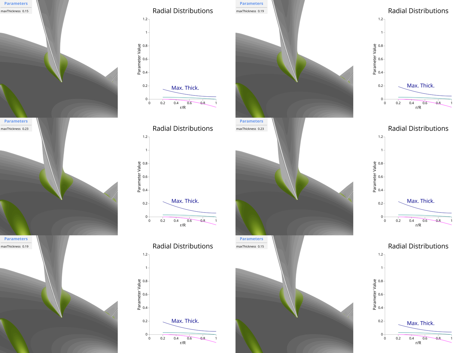
The Max. Thickness distribution describes the maximum thickness of each profile in the chordwise direction. This function is controlled by a single design variable named maxThickness_00.

• Set the range of maxThickness_00 from 0.15 to 0.25, with a default value of 0.2.
• Convert maxThickness_01 and maxThickness_02 to parameters and set them to maxThickness_00 * 0.25.
  • This is designed to achieve the greatest thickness in the spanwise direction at the root of the blade, gradually decreasing towards the tip.

In the animation below, you can see the effect of the maxThickness_00 parameter on the propeller model.

Trailing Edge Thickness

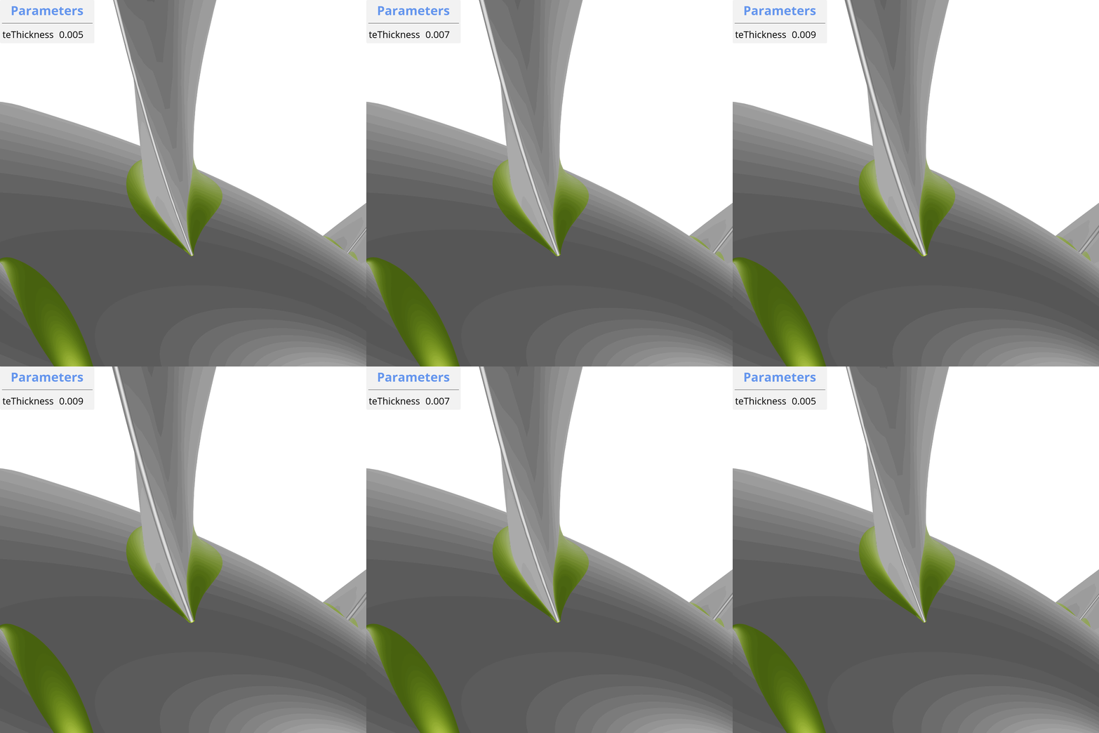
For the Trailing Edge (TE) Thickness distribution, a constant distribution will be used, so the plus button will not be clicked.

• Create a new design variable named teThickness under the Functions scope.
• Set the range of teThickness from 0.005 to 0.01, with a default value of 0.0075.
  • This is designed to maintain a constant TE thickness.

Angle of Attack

note

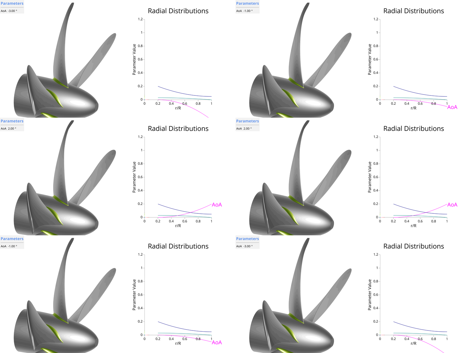
It is an optional step to add a distribution function for the angle of attack, which is preferably used when a tip rake is added to the propeller blade.

The Angle of Attack distribution describes the rotation profile by changing the angle of attack. This function is controlled by a single design variable named angleOfAttack_02. It is designed to twist the blade's profile to both negative and positive values, with zero representing no twist.

• Set the range of angleOfAttack_02 from -0.3 to 0.3, with a default value of 0.
• Convert angleOfAttack_00 and angleOfAttack_01 to parameters and set them to 0.
  • This is designed to achieve the greatest twist in the spanwise direction at the tip of the blade, gradually decreasing towards the root, where there is no twist.

Under the Profile Parameter for angleOfAttack distribution, you need to scale up this distribution by a factor of 10, as follows:

[|propeller|blade|functions|angleOfAttack_distribution|angleOfAttack_distribution, 10].

In the animation below, you can see the effect of the AoA parameter (angleOfAttack_02 * 10 in degrees) on the propeller model.

All 2D Radial Distributions

Below is a figure showing all 2D radial distributions, including those from the Center Surface and those from the Profile Parameters.

note

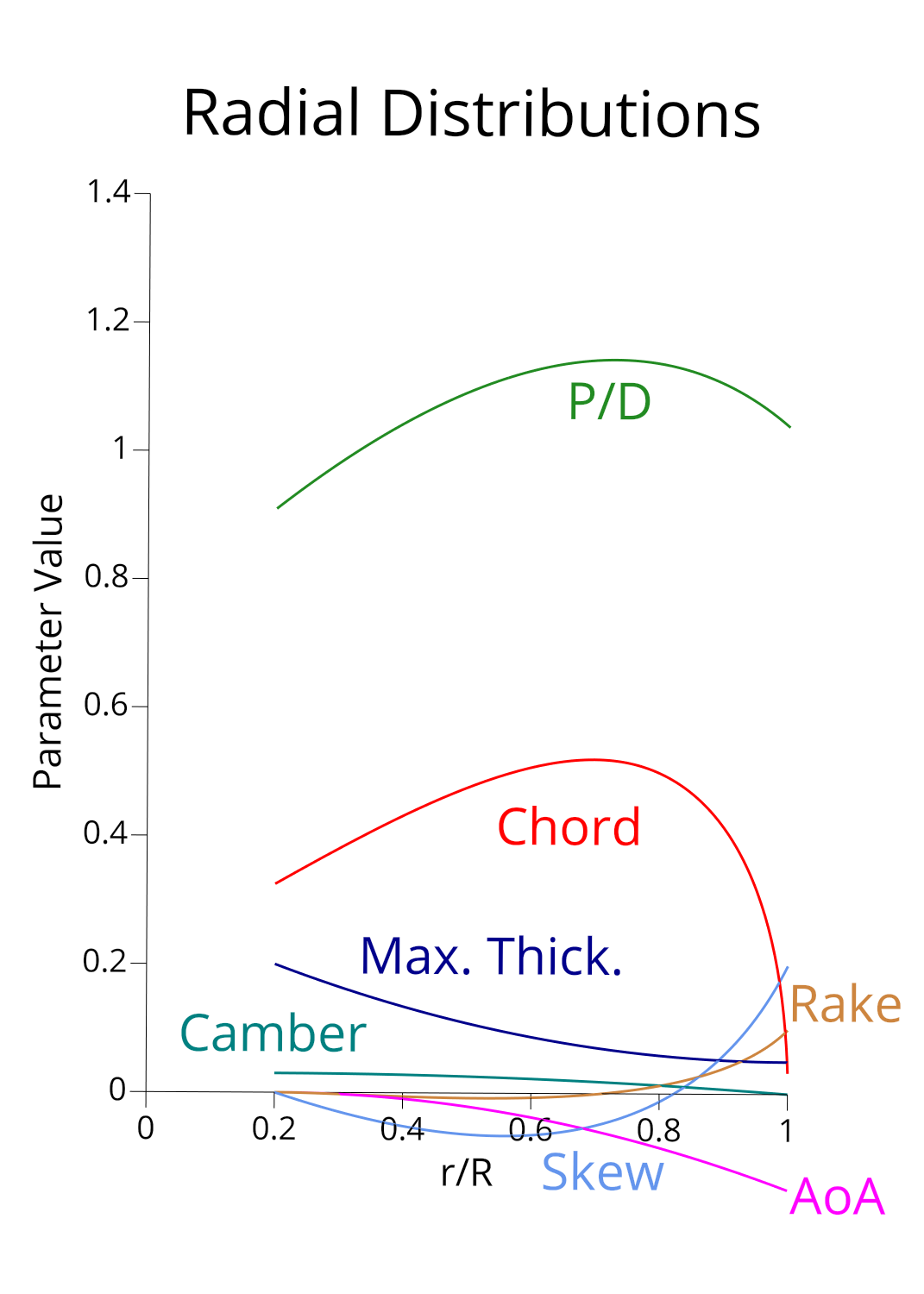
For all Profile Parameter Distributions, you need to adjust the X positions of the points p00, p01 and p02.

• p00:X = |propellerAdvanced|00_functions|radiusHub
• p02:X = |propellerAdvanced|00_functions|radiusTip
• p01:X = (p00:X + p02:X) / 2

Final Blade Surface

The bladePrepared is an ImageSurface that is automatically configured by the workflow. Below, the properties of the bladePrepared are shown:

• Source: blade
• U-parameters: [0, 1]
• V-parameters: [0, 1 - |propeller|blade|tipGap]

The V-Domain setting of the blade surface makes room for a closed tip surface, which will be addressed in the next step.

Tip Surface

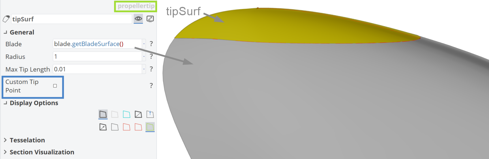
Here, the Tip Surface is created by clicking the plus button in the propeller component GUI. The following properties are automatically configured for this setup:

• Source: |propeller.getBladeSurface().getBladeSurface()
• Radius: 1
• Max Tip Length: 0.01

Below is a figure showing the tip region of the blade. The main part of the blade is depicted in gray , while the tip surface is highlighted in yellow color.

Propeller Solid

Following the creation of the blade and tip surfaces, the next step is to create a watertight, closed solid geometry.

• Click the plus button corresponding to the Propeller Solid in the propeller component.
  • This will generate a bladeSolid component along with two design variables named absPropellerRadius and NOB.
  • These correspond to the propeller radius and the number of blades (NOB).
• Set the range of absPropellerRadius from 100 to 5000 millimeters, with a default value of 2500.
• Keep the range of NOB from 3 to 5, with a default value of 3.
  • Set it as an integer design variable by toggling the Integer check box.
• Next, create a parameter under the bladeSolid component named "D" for Diameter.
  • Set the expression of D to: absPropellerRadius * 2.

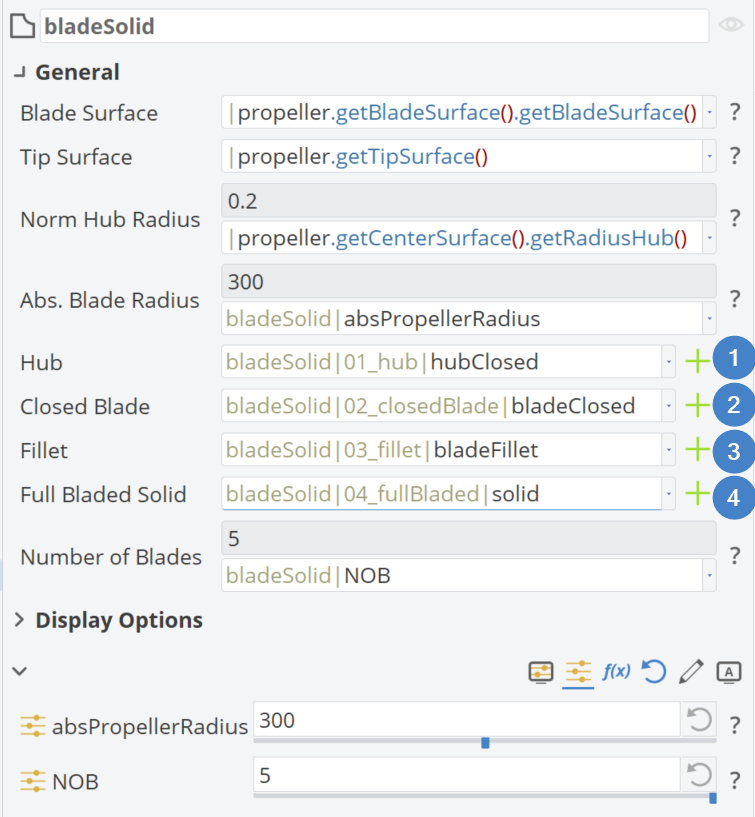
Steps for Propeller Solid Creation

The steps to complete these tasks are illustrated in the figure below.

Hub

By clicking the corresponding plus button in the bladeSolid GUI, you can create a hub BRep scaled to the propeller's radius. For this tutorial, the auto-configured hub from the workflow is sufficient. However, if you wish to make adjustments, an easy modification is to adjust the axial length of the hub using the following parameter. This keeps the length relative to the propeller's radius by adjusting the factor 0.75:

axialLength = |propeller|bladeSolid.getBladeRadius() * 0.75

Closed Blade

Afterward, you can create a Closed Blade as a BRep in a similar manner. This is achieved through an Operation: boolean|solid from intersections of a scaled version of the blade & tip surface to the propeller radius, combined with a scaled-down version (99%) of the hub geometry, named hubSmall.

Variable Radius Fillet

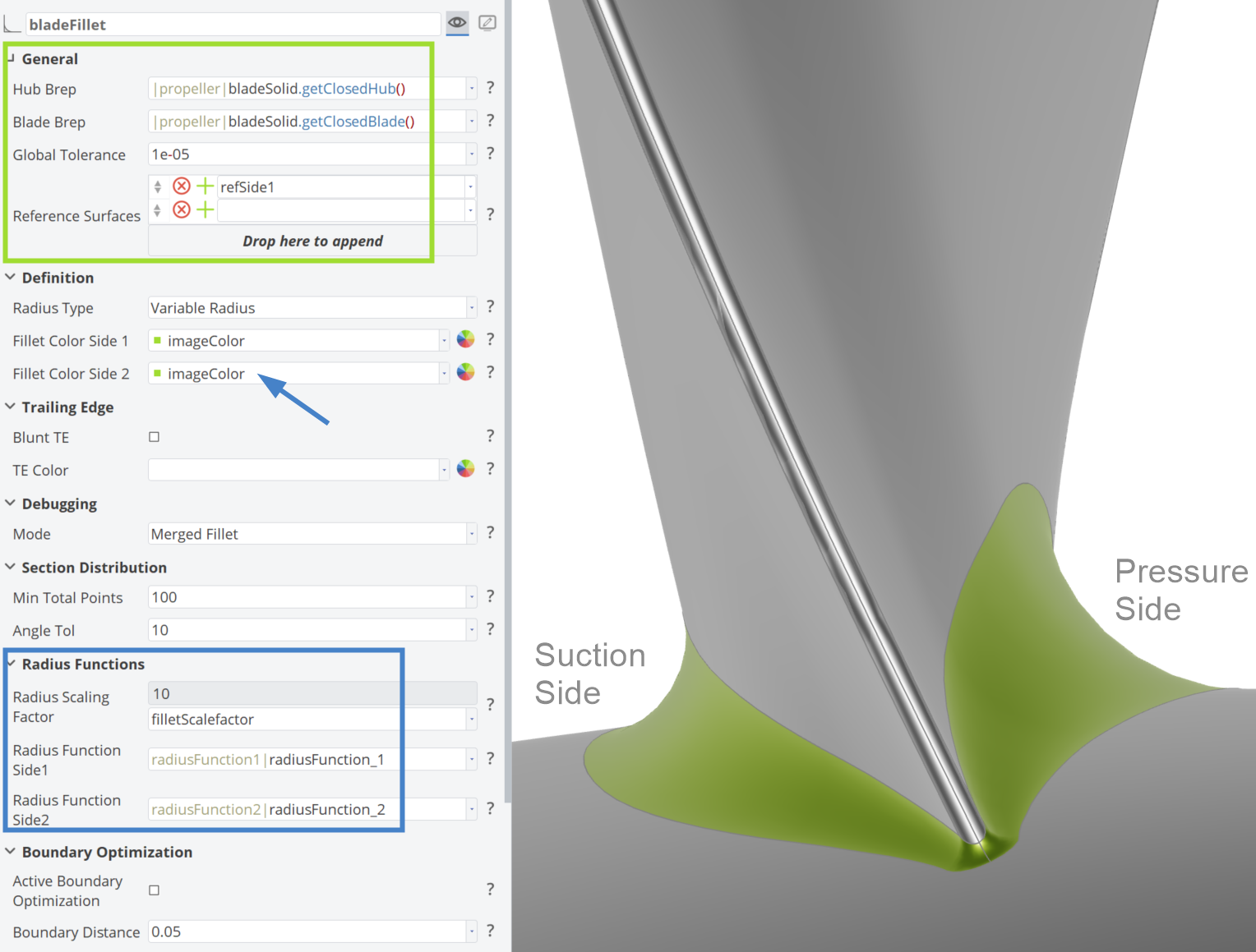
Having BReps for the blade and the hub correspondingly, then we can move on to the Variable Fillet creation. A rule of thumb that we use for the fillet is to set the fillet radius on the pressure side to 2/3 of the maximum profile thickness at the root and 1/3 on the suction side accordingly. Also, the fillet should follow the thickness at the TE and the LE. Based on the aforementioned the following Parameters are defined:

• filletScalefactor = 10
• radiusLe = thicknessRoot / 10
• radiusSide1 = thicknessRoot / 3
• radiusSide2 = thicknessRoot * 2 / 3
• radiusTe = thicknessTE / 2
• thicknessRoot = |propellerAdvanced|00_functions|04_chord|chordRoot * |propellerAdvanced|blade|functions|maxThickness_distribution|maxThickness_00 * |propellerAdvanced|bladeSolid|D
• thicknessΤe = |propellerAdvanced|00_functions|04_chord|chordRoot * |propellerAdvanced|blade|functions|teThickness * |propellerAdvanced|bladeSolid|D

The following image shows the GUI of Variable Fillet.

Final Full Bladed Solid

The final step of the Propeller Solid is to create the complete propeller geometry, with all blades smoothly connected to the hub as a single BRep.

• Click on the plus button next to Full Bladed Solid and the workflow will create a watertight solid automatically.

In the animation below, you can see the effect of the NOB parameter on the propeller model.

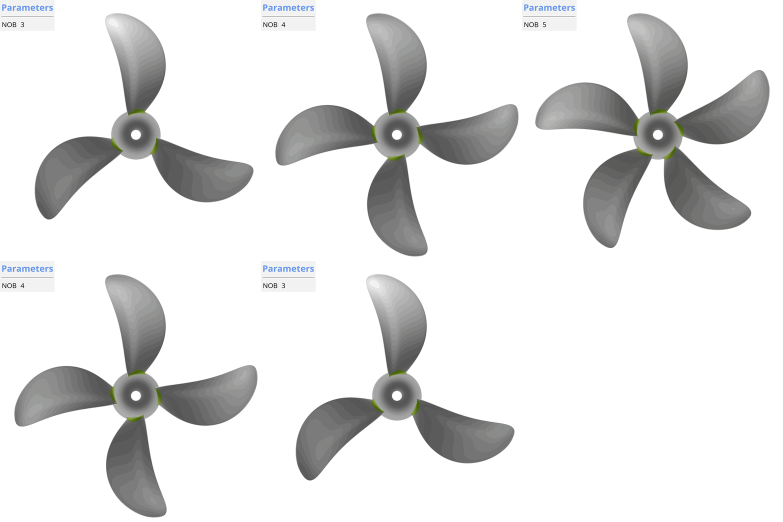
This concludes the modeling of the propeller. The next step, is to connect this model to a CFD RANS solver and automatically create a Flow Domain.

Flow Domain

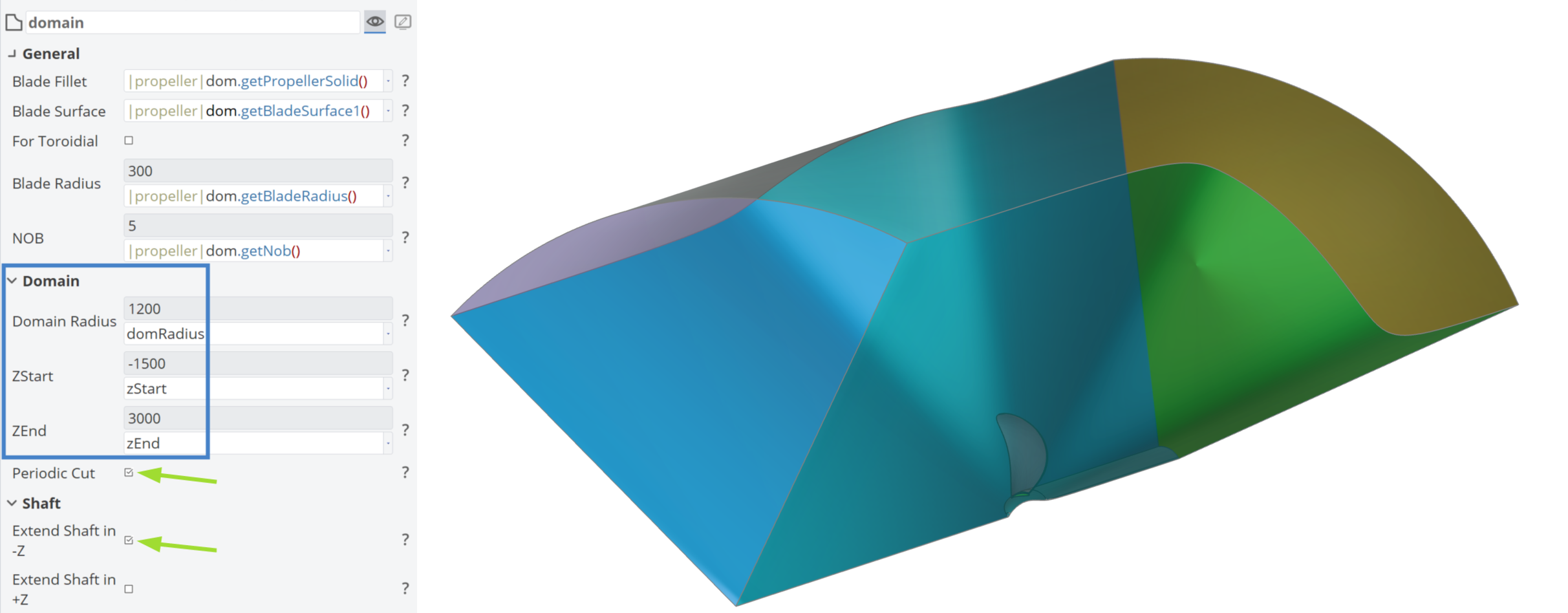
For the propeller's Flow Domain you can click the plus button from propeller component GUI and then do the same to the pop-up dom component. Then if you unfold the dom you may find the dom|domain Object and following parameters:

• domRadius = |propeller|dom.getBladeRadius() * 4
• zEnd = |propeller|dom.getBladeRadius() * 10
• zStart = -|propeller|dom.getBladeRadius() * 5

You can adjust the parameters according to your preference, but it is recommended to keep them relative to |propeller|dom.getBladeRadius().

One Blade Segment

The checkbox Periodic Cut should be checked to include only one blade in the domain, resulting in a smaller problem to solve.

note

If your solver does not assume symmetry, leave the Periodic Cut checkbox unchecked. Similarly, you may check the Extend in -Z Axis option if it better suits your setup.

Conclusion

This tutorial aims to help you become more familiar with the Advanced Propeller Workflow and demonstrates how to modify some of the default settings, allowing you to see firsthand how easy it is to do so. You can also adjust your own workflow to align with CAESES. Additionally, a parametric model is introduced here with a few parameters to maintain a compact design space, enabling meaningful designs while also providing the freedom, flexibility and variety needed for both conventional and unconventional propellers (such as highly skewed and tip-rake designs).

---

Final Setup

CAESES Project File

If you want to take a look at the finalized parametric model you can find the resulting CAESES project file advanced-propeller-workflow.cdb here:

Load Final Model