Parametric Profile Design

In CAESES, profiles can be defined in various ways. Basically, any curve type of CAESES can be used to set up a blade profile description. Typically, mathematical descriptions are used, for instance NACA formulas etc. This tutorial gives you an example of a parametric profile design where such a mathematical definition is involved.

See also the sample section where you can also find an axial blade design which is based on an offset curve, using a mean camber definition plus a thickness distribution.

Finally, if you want to design axial blades for compressors with rather complex i.e. curved meridional contours, then see the corresponding tutorial and samples for these types of turbomachinery.

For demonstration purposes and to keep it simple, a mean line camber of a NACA 4-digit airfoil is defined in this tutorial. This will give you the basic idea of how to create your own mathematical definitions. Prerequisites for this example are the Feature Tutorials.

Generic Curve

The Generic Curve allows you to define a parametric curve. The reserved parameter of this curve type is called t: It internally runs from 0 to 1 so that a curve can be generated. In this step we'll have a quick look at the Generic Curve in order to understand the parameter t.

• Let's create a Generic Curve via Model workspace > CAD tab > Curves category > More > Generic.

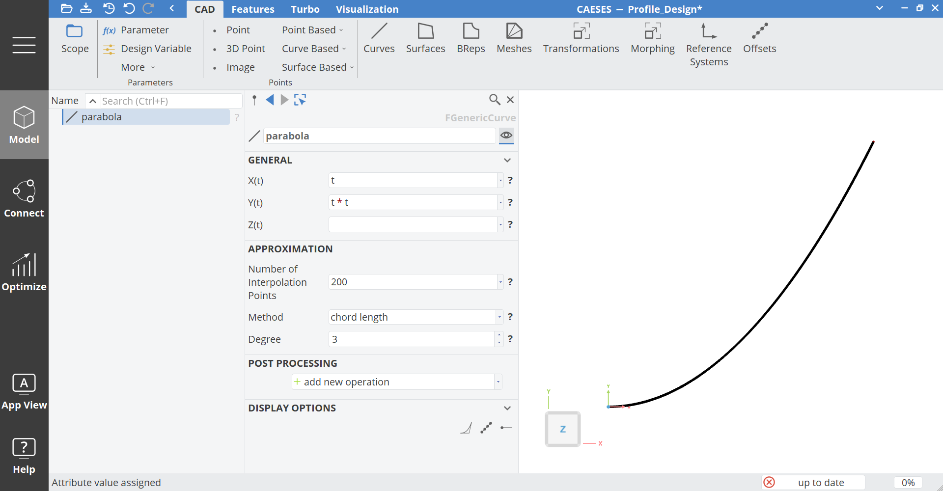
• Change the name from genericCurve1 to "parabola"

• Enter t into the attribute X(t).

• Enter t*t into the attribute Y(t).

• Try out other expressions for Y(t) such as sin(t*360).

• Delete the curve -- we do not need it anymore for the next steps.

New Feature Definition

The mean camber line will be defined within a Feature Definition. This will give you a first idea of how to define your own formulas. In this step, the arguments are configured:

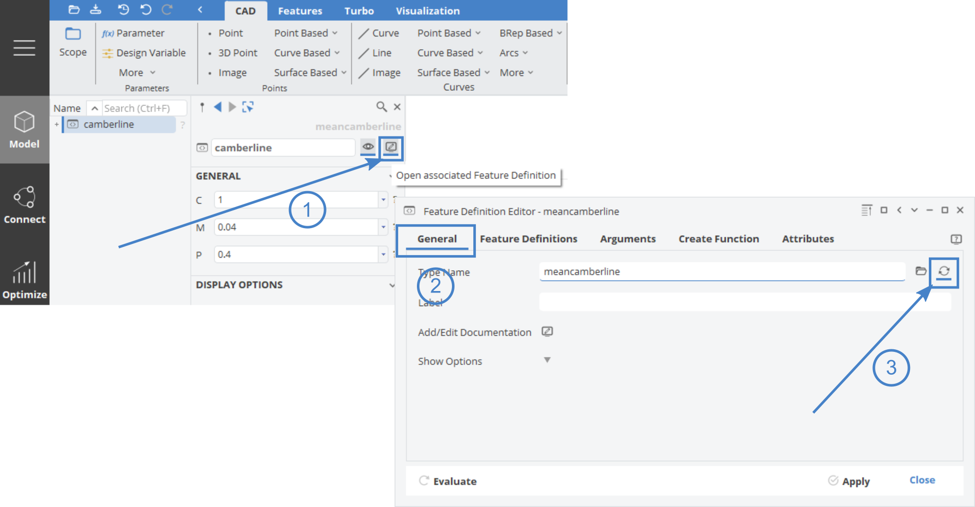
• Go to Model workspace > Features tab > Create Definition.

• Enter "meancamberline" in the Type Name attribute (General Tab of Feature Definition Editor).

The NACA mean camber line requires 3 input values:

• chord ("c"),
• maximum camber ("m")
• and the location of maximum camber ("p").

Here is the definition:

$$y_c=\left\{ \begin{array}{l} m\frac{x}{p^2} \left( 2p-\frac{x}{c}\right) \qquad \text{for} \quad 0\leq x \leq pc \\ \\ m \frac{c-x}{(1-p)^2}\left( 1+\frac{x}{c}-2p\right) \qquad \text{for} \quad pc \le x \leq c \end{array} \right.$$

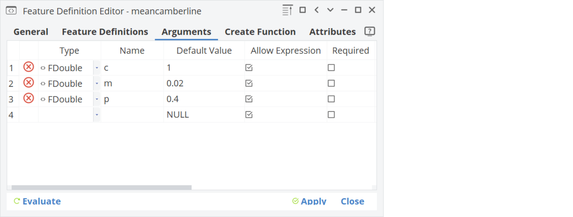
• Go to the Arguments tab in the Feature Definition Editor and add the 3 input arguments. Choose FDouble for the Type.

• Set default values according to the screenshot.

Formula

The formula for the mean camber line is now put into a Generic Curve.

note

The curve parameter t corresponds to x in the formula and t runs from 0 to 1. Therefore, we have to multiply t with the chord length.

• Paste this sequence into the Create Function editor, press Apply and close the dialog:

parameter tc(t*c)  
parameter pc(p*c)  
genericcurve mean()  
mean.setX(tc)  
mean.sety( \
    if( tc<pc, \
    m*tc/(p*p)*(2*p-tc/c), \
    m*(c-tc)/(1-p)^2*(1+tc/c-2*p)) \
)

tip

Long expressions can be separated by using the \ character. You can also write it in one line:

parameter tc(t*c)  
parameter pc(p*c)  
genericcurve mean()

mean.setX(tc)  
mean.sety(if( tc<pc, m*tc/(p*p)*(2*p-tc/c), m*(c-tc)/(1-p)^2*(1+tc/c-2*p)))

The if-statement in this expression is also a Global Command in CAESES.

Testing and Export

Let's create a feature from our new definition to check whether everything works correctly.

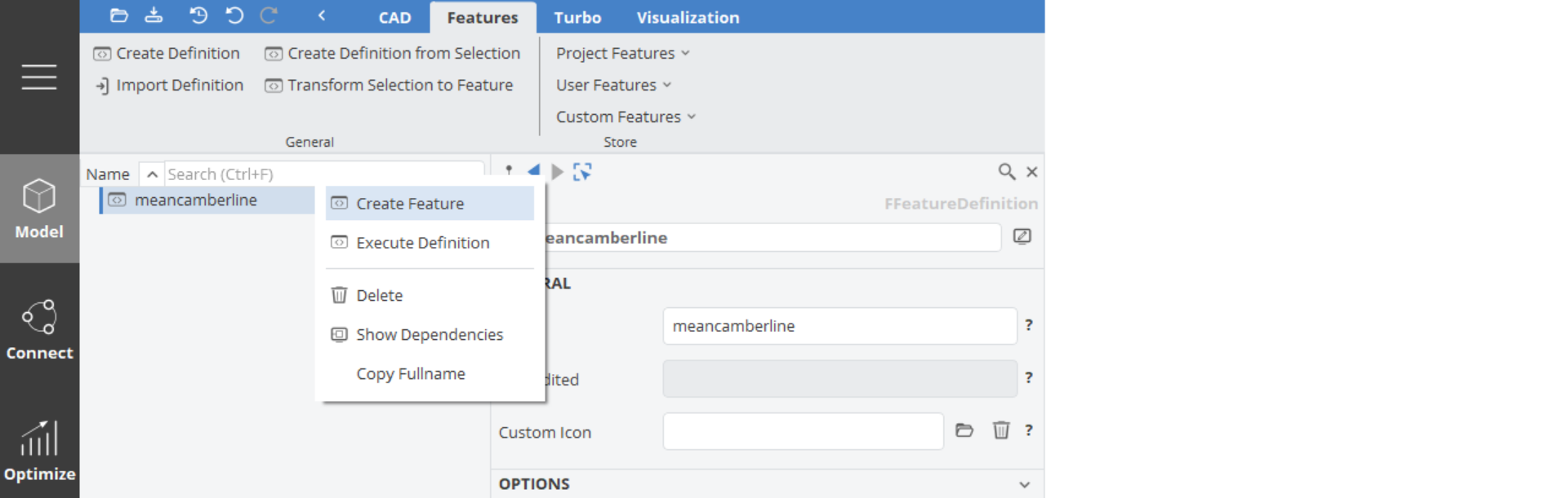
• Create a Feature via the context menu (right-click) of the definition in the tree. (Model workspace > Feature tab).

• Switch to the CAD tab to see the created feature

• Rename the new feature meancamberline1 to "camberline".

• Change the input values C, M and P to check the curve in the 3D view.

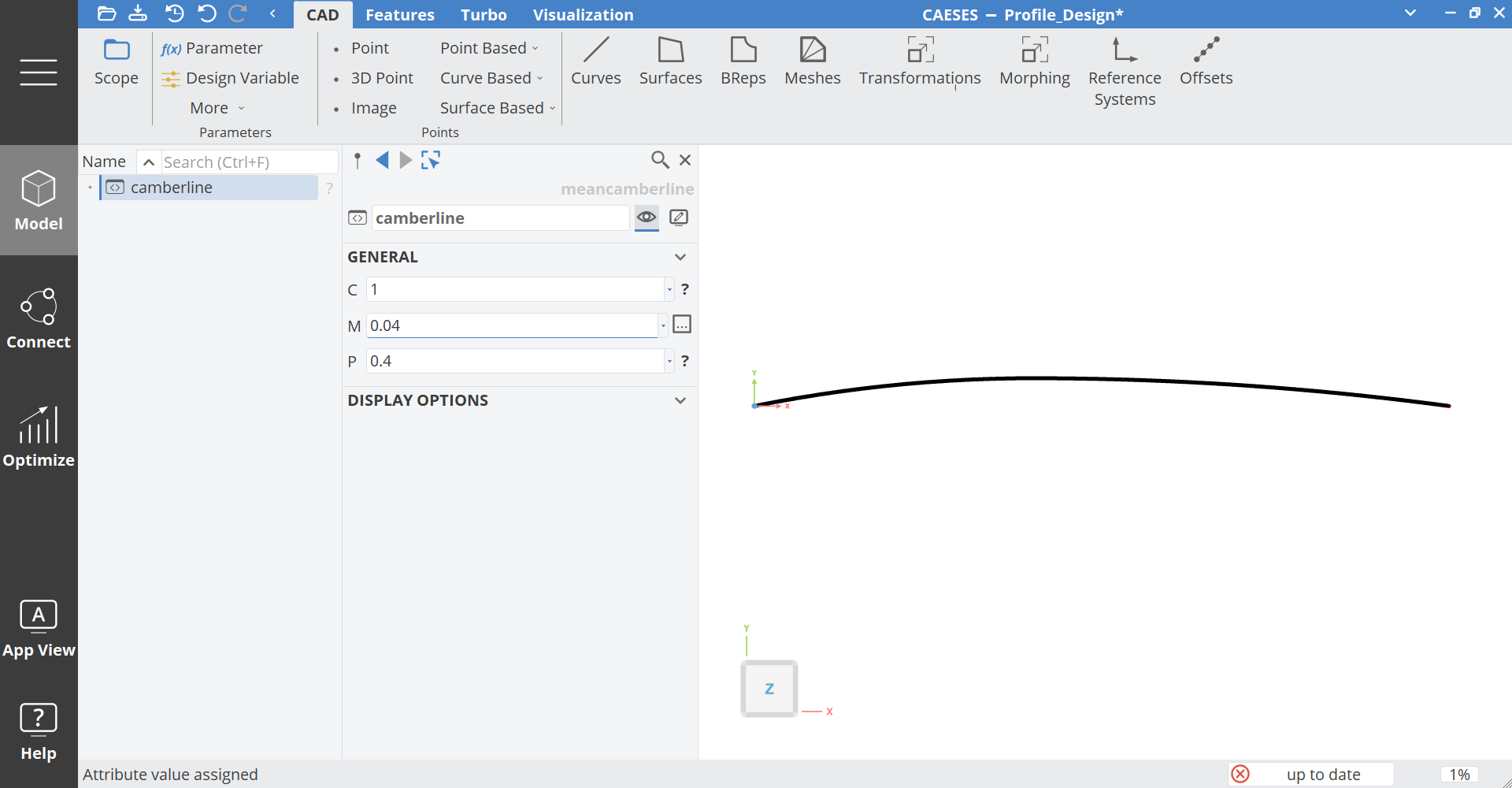
• Set the chord (C) value to 1 -- we won't change it in this tutorial.

Optional: Export the definition so that you can access it again from other projects via the menu features > in user directory (helpful for recurring usage of the same definitions). The export option can be found in the General tab of the Feature Editor.

Profile Modeling

Thickness Distribution

In order to create a profile that is based on our mean camber line, we first need a simple thickness distribution.

Let's create an F-Spline curve for our thickness distribution:

• Choose Model > CAD > Curves > Point Based > F-Spline and name the new curve "thickness".

• Set the Start Position to [0,0,0].

• Set the Start Tangent to 90.

• Set the End Position to [1,0,0].

• Set the Area Value to 0.04.

• Set the curve's color to red (in the category Display Options).

note

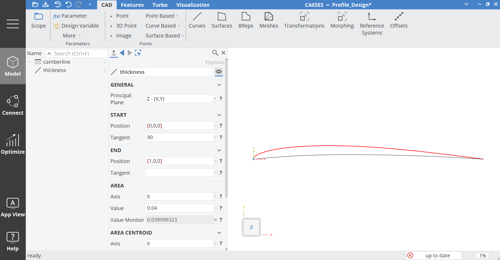
We need a normalized thickness distribution in the X-interval [0,1] for the next step.

Offset Curve

So far, a camber mean line and a thickness distribution are given. The profile curve is now created by means of an Offset Curve.

• Go to Model > CAD > Curves > Curve Based > Offset and name the new curve "profile".

• For the Curve attribute, set mean from the Feature camberline. Choose it from the drop down menu or drag and drop the mean curve into the field. (Click the little + icon in front of the camberline to expand it.)

• Set the curve thickness for the attribute Thickness Distribution.

• Click on the General category to see further options.

• Set the LE (leading Edge) Blend Position to 0.03.

• Activate Both Sides in the Offset Options category.

tip

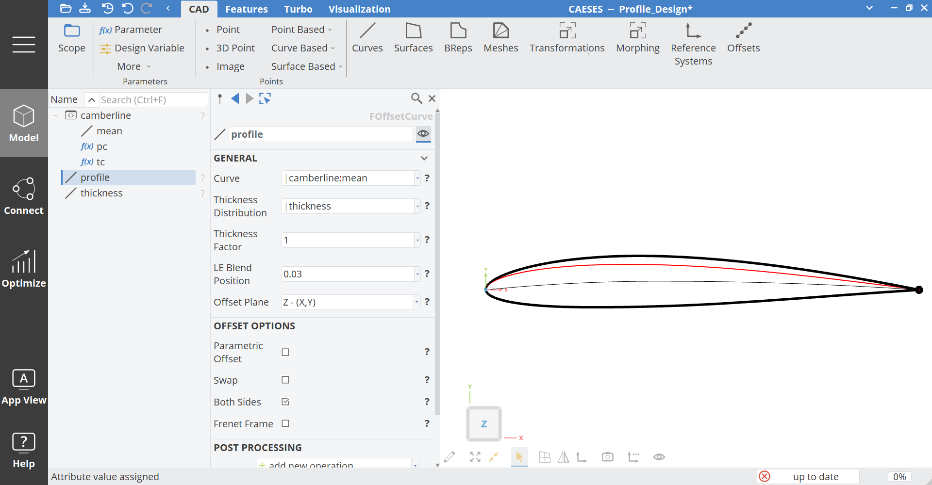
When you specify a leading edge (LE) blend position, the offset curve can consider this information during the curve generation process. This results in better 2D and 3D shapes of the profiles.

Check out the Axial Fan Sample where you can find an axial blade whose profile is based on the presented design approach.

---

Final Setup

CAESES Project File

If you want to take a look at the finalized parametric model you can find the resulting CAESES project file profile-design.cdb here:

Load Final Model