Dimensionality Reduction with Principal Component Analysis
The dimensionality reduction method is used to speed-up the optimization process of complex geometries with many design variables. It helps to reduce the number of free design variables that are used for the optimization procedure, while only scarifying a small portion of the model's variability.
Often sophisticated parametric models are set up with a large number of design variables, that make the optimization task difficult and require a lot of computational resources. Design spaces typically consist of many dimensions since complex shapes require a lot of design variables to define them suitably. Each additional design variable adds another dimension to design space. The higher a system’s degree-of-freedom (free design variables) the more simulations are usually needed to understand the system and to find improved designs. Faster optimizations come from intelligently reducing the degrees-of-freedom (free design variables) and, as a consequence, cutting down the necessary number of simulation runs.
Typical Design Variables, even though chosen with care from a diligently crafted parametric model, still influence certain regions of a shape similarly, leading to unwanted dependencies. Those unwanted dependencies are detected and eliminated by the dimensionality reduction method.
In this tutorial we will use the dimensionality reduction method to show how the number of free design variables can be decreased, while keeping most of the model's variability. We will use an S-duct model which is complicated enough to illustrate all necessary steps yet easy enough to follow.
Open S-Duct Model as a Starting Point
Let's get started by opening an existing s-duct model, which will be our starting point for this tutorial.
Get started with the project file s-duct_starting_point.cdb and open the s-duct model.
- Save the project in a directory of you choice by clicking on the Menu workspace > File tab > Save project as, so that we don't overwrite the existing model.
Original Design Variables
The s-duct shape is varied by 14 Design Variables, that influence the height, width and weight of the cross sections along the path. Take a look at the different Design Variables of the s-duct.
- In the Model workspace > CAD tab click on the Design Variable icon next to the 01_functions scope to see an overview of all Design Variables.
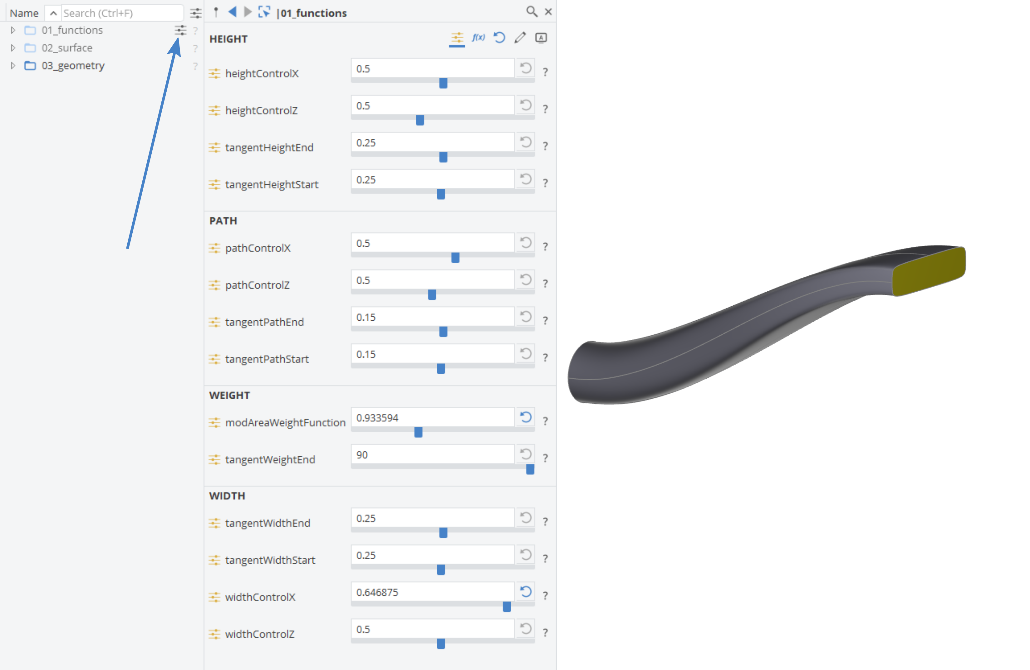
- Move the sliders of all Design Variables to get familiar with the modifications.
Usually we would select a subset of all available Design Variables to use them in the optimization depending on available computational resources. In this case we do not choose certain Design Variables but rather put all of them in the Dimensionality Reduction method to see what the most influential Principal Parameters are.
Setting up the Dimensionality Reduction
- Go to the Optimize workspace > Optimization tab > Design Space Utilities and create a Dimensionality Reduction.
Create a Sample Set
Now we want to create a large variation of the duct geometry and run a pure geometrical DoE (without any CFD computation).
In the Dimensionality Reduction:
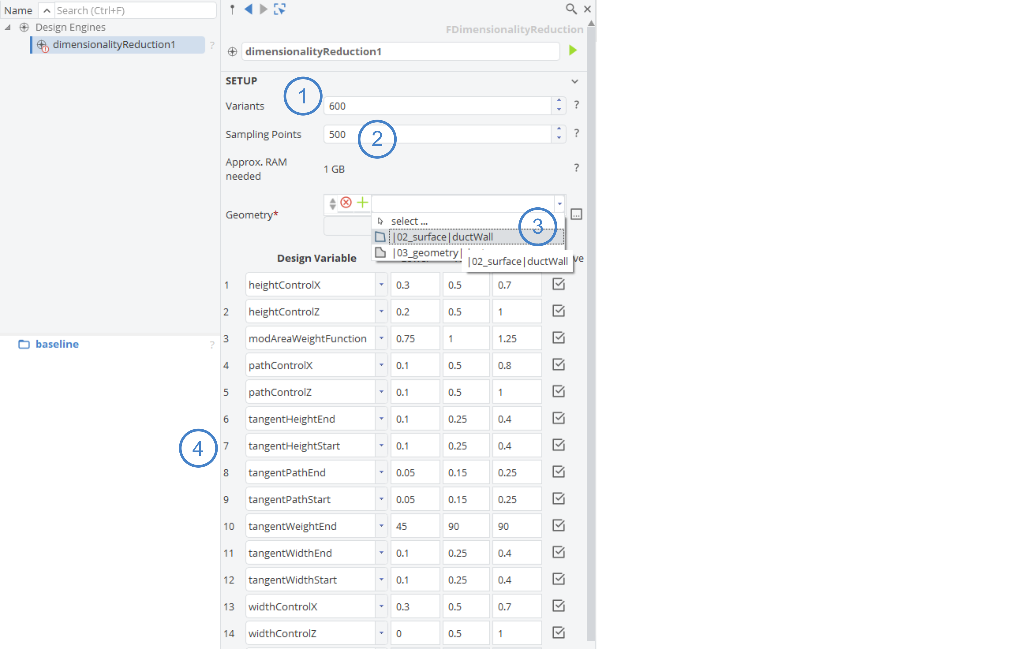
- Set the number of Samples to
600. - Set the number of Points per Sample to
500. - Set the ductWall as the input Geometry by choosing it from the drop down menu in the Geometry field.
- Set all 14 Design Variables at the bottom. You can choose them one by one from the drop-down list and add every available Design Variable to the setup.
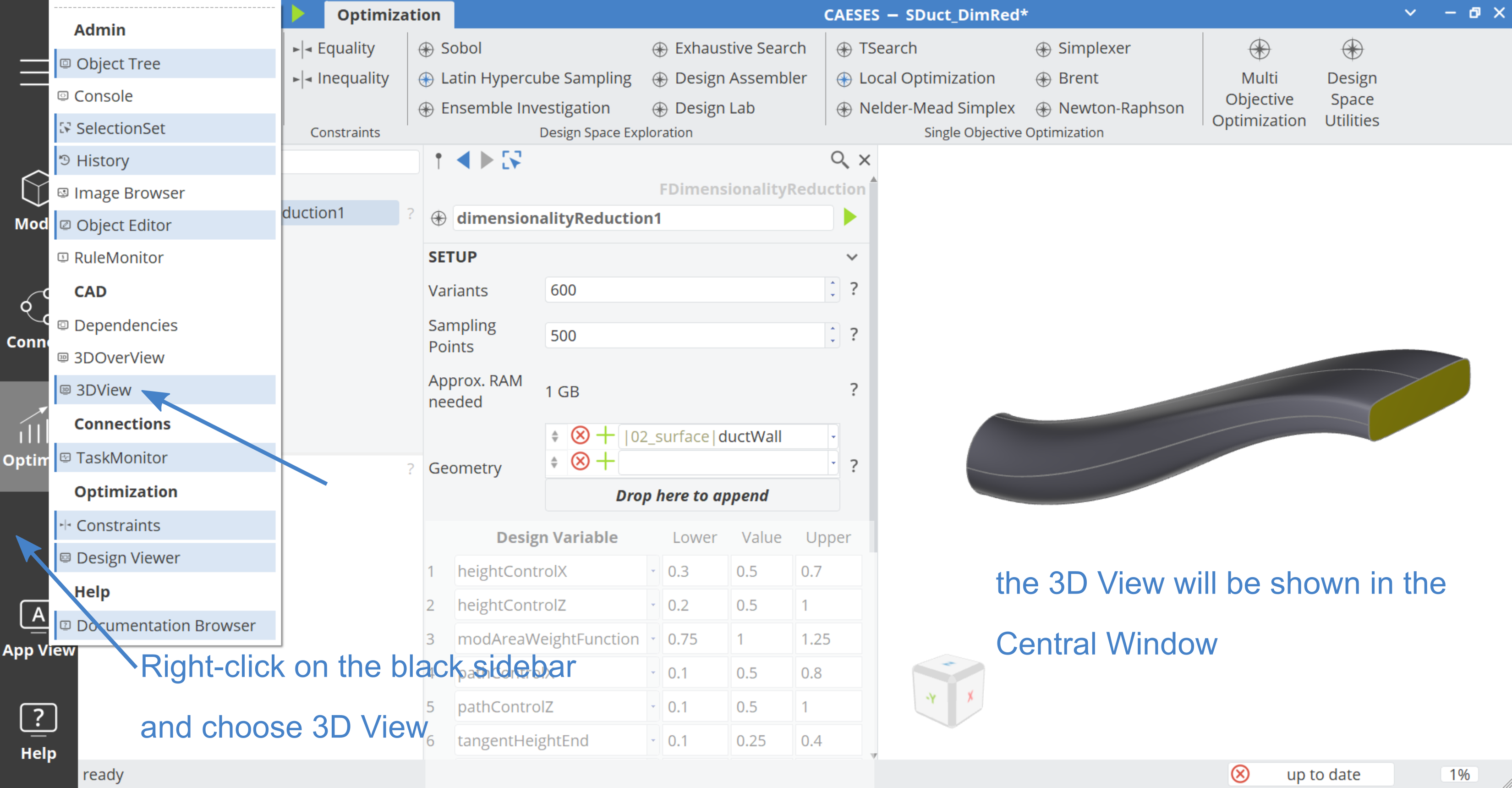
Since we are in the Optimize workspace the 3D View is not visible (by default) in the Central Window.
- Open the 3D View by clicking on the black workspace sidebar with the right mouse button and choose 3D view from the list.
Let's run the dimensionality reduction and let it create the 600 shape samples. Depending on the complexity of the model this sample variant creation is quite fast, since no CFD simulation needs to take place at this point. It is a pure geometrical Design-of-Experiment (Sobol) creating the sample variants.
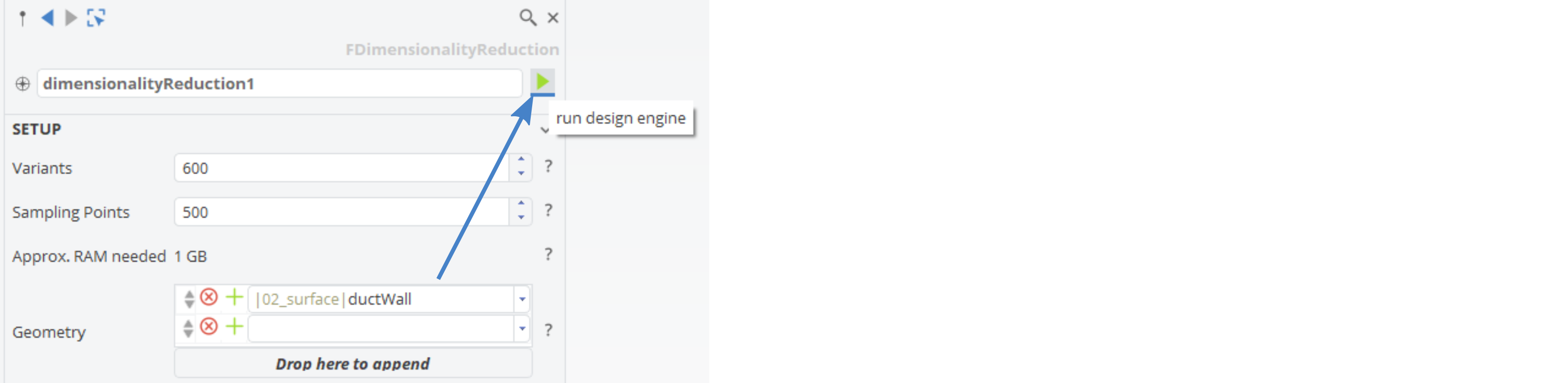
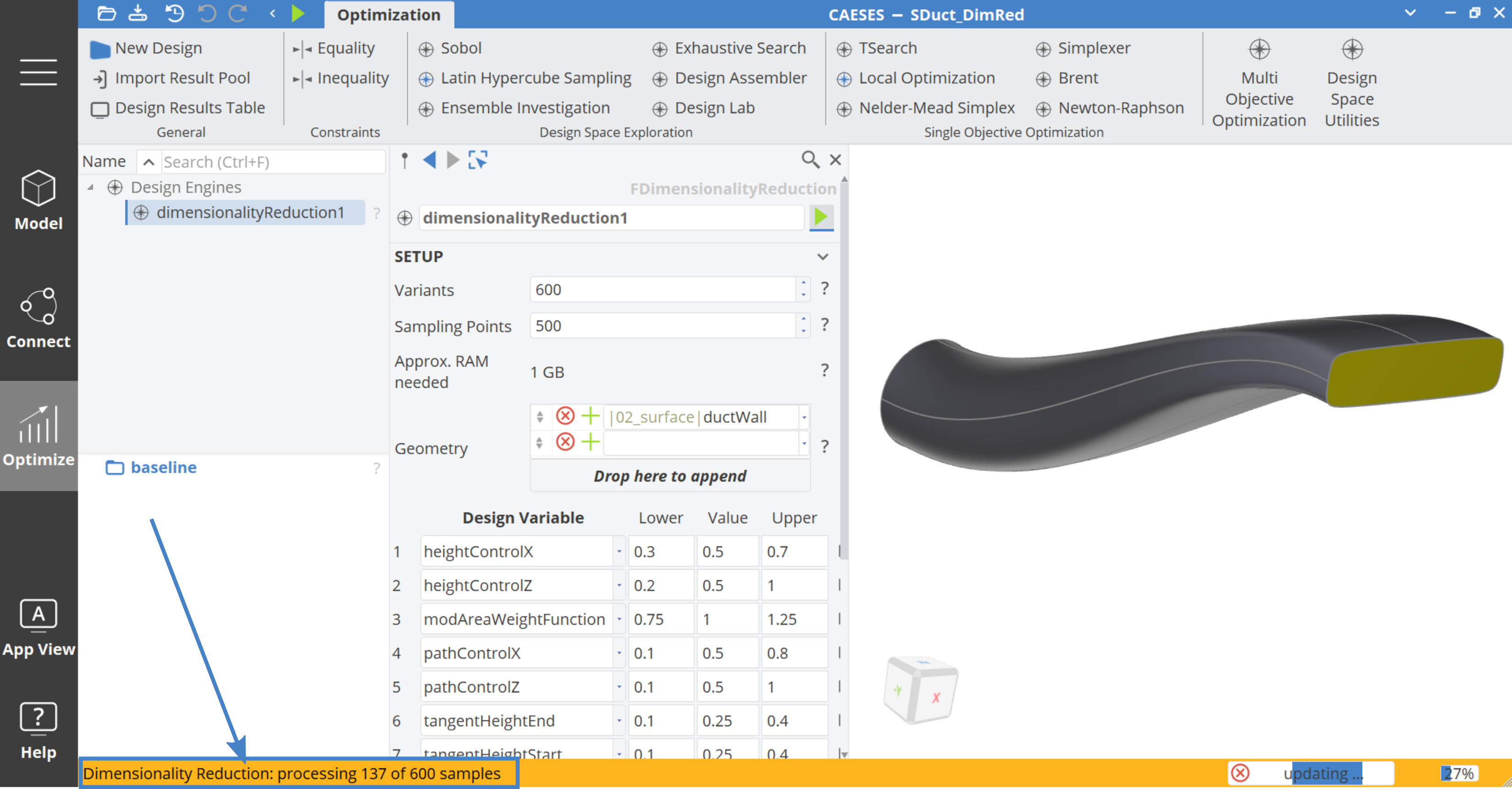
This process takes a few minutes. While the internal Design Creation is running a yellow bar appears at the bottom of the interface that tells you how many samples have been created. The Principal Parameters will be derived from the sample variants created in this internal Design Exploration (Sobol) run.
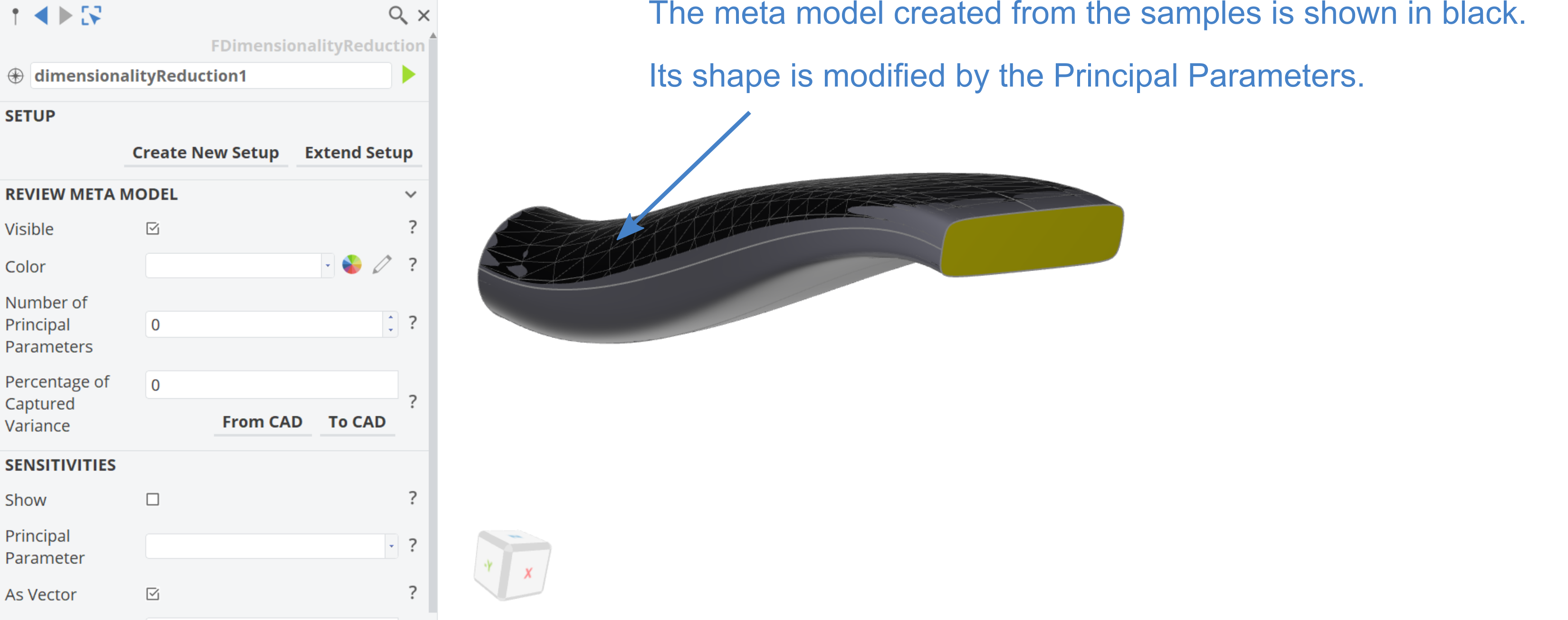
When the sampling process was completed successfully the meta model becomes visible in the 3D view (a black surface with the number of discretization points we defined in the Points per Sample attribute). Also the Object Editor now shows the options to set a number of Principal Parameters and to visualize them in the 3D view.
Analyze the Principal Parameters
Let's take a closer look at the Principal Parameters that were derived from the sample set.
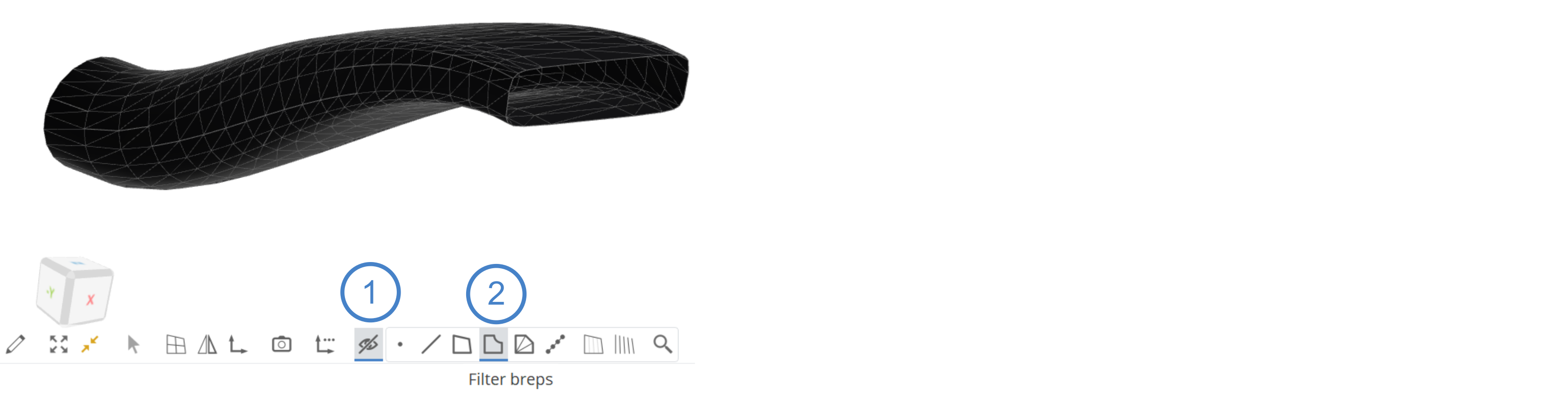
- Hide the original s-duct model by activating the BRep filter in the 3D view
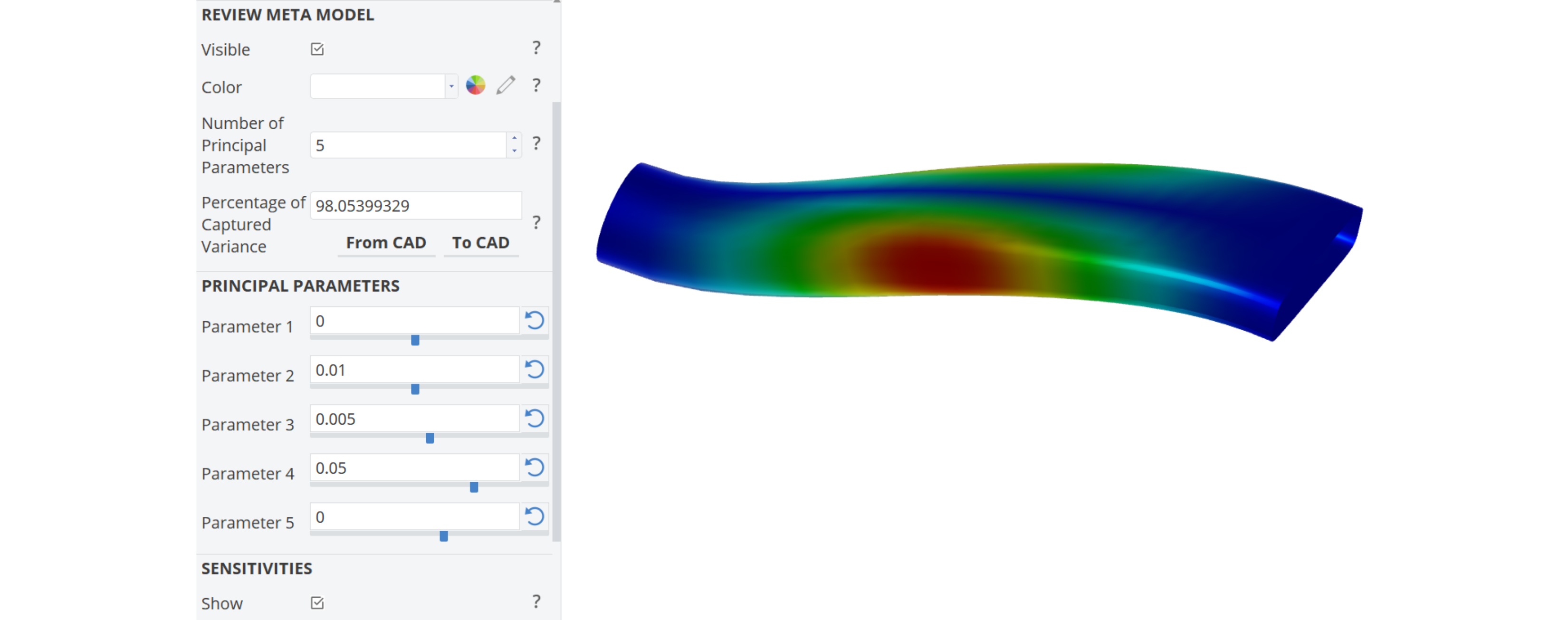
- Set the Number of Principal Parameters to
1. The field below now shows the percentage of captured variance or variability of the meta model if we continue with a single Principal Parameter. - Increase the Number of Principal Parameters step by step and see how the captured variance percentage changes with each additional Principal Parameter that is taken into account.
Setting the Number of Principal Parameters to 4 would already result in 96% of the variability of the original model, captured with just four Principal Parameters.
- Move the sliders of the Principal Parameters to see how the meta model changes its shape in the 3D view.

Visualize Sensitivities of Principal Parameters
To visualize what particular region is influenced by the different Principal Parameters toggle the Show button in the Sensitivities category and set a Parameter you would like to visualize.
If you activate the As Vector option you can visualize the vectors for each discretization point that indicate how the point is moved by the Principal Parameter.
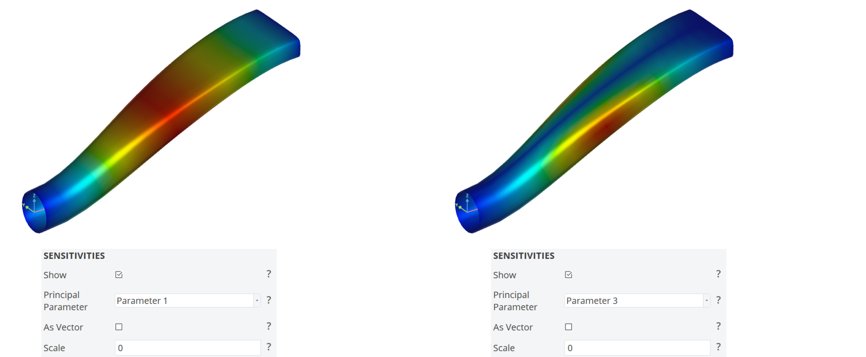
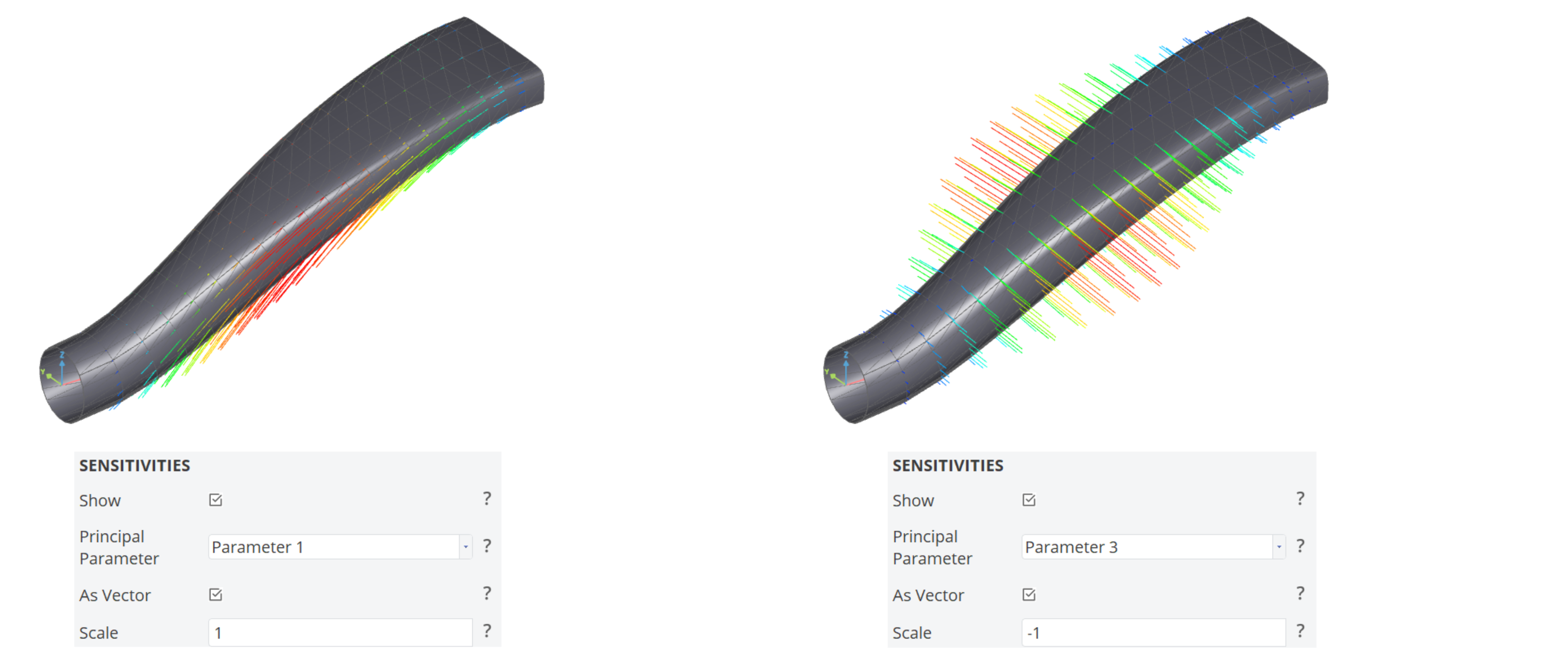
Let's disable the sensitivities again by toggling the Show button in the Sensitivities category.
Testing the Dimensionality Reduction Meta Model
Each shape that is described by the meta model (shown in black) and the Principal Parameters needs to undergo a Back-Transformation, since in the end we want to work with the original model and ensure the BRep quality for further steps.
To test the setup the buttons From CAD and To CAD come into play.
Find Principal Parameter Values
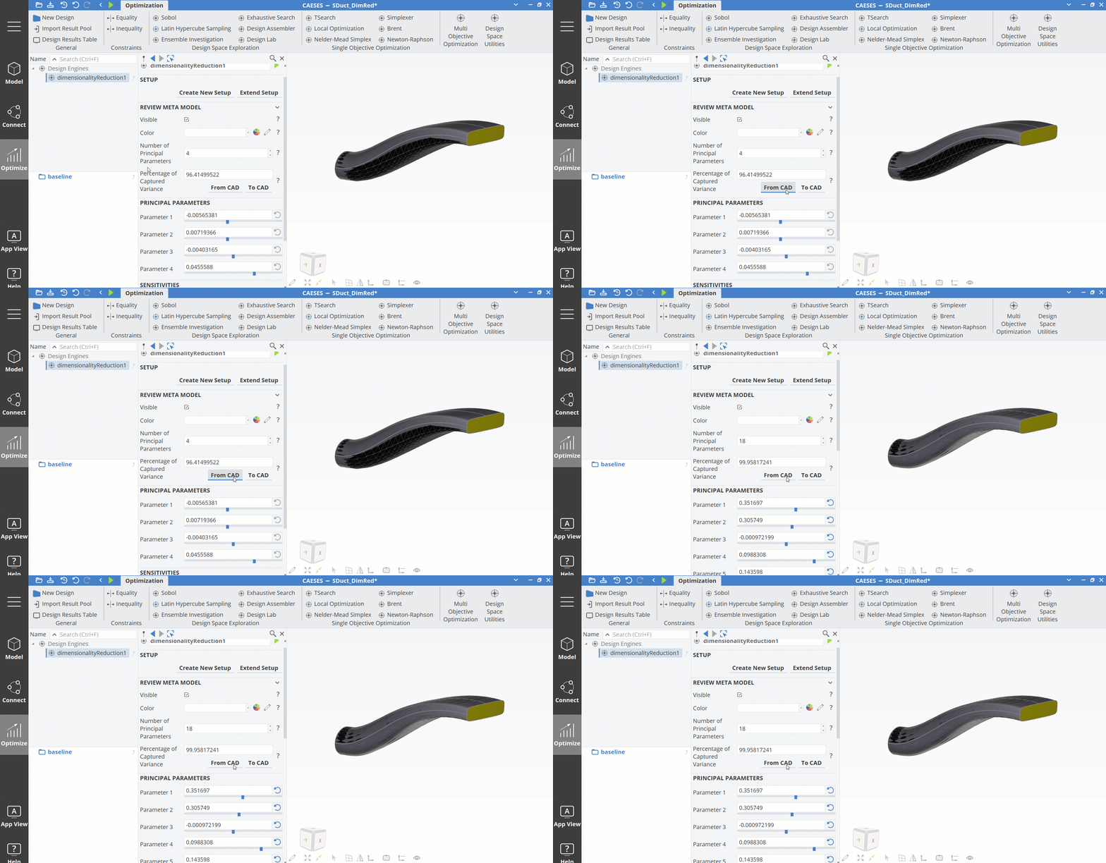
The From CAD button finds the Principal Parameter values for the current original design variable setting.
- Make the BRep visible again by disabling the BRep filter at the bottom of the 3D view.
The original duct model should be visible again now.
If you want to map the meta model to lay on top of your original geometry, click the From CAD button. The values for each Principal Parameter are calculated and set in the Object Editor and the meta model shape "jumps" onto the original shape.
Reconstruct Original Design Variables (Back-Transformation)
The back-transformation means that the values of the original design variables need to be found which (best) fit the shape defined by the chosen number of Principal Parameters.
The main difficulty of reconstructing the design variables of the original CAD model for any new shape given by the Principal Components is that an explicit mathematical relationship between the CAD space and the new Principal Parameter space is not available. By omitting some of the less important Principal Parameters, information (variability) is lost and deliberately sacrificed to lower the total number of free variables for the optimization process. This makes it harder to reconstruct the correct design variable values, which is where some deviations come in.
A back-transformation is done automatically after each automated variant creation, if you use the Principal Parameters in a Design Engine.
The To CAD button finds the original design variable values for the current Principal Parameter setting (triggers the back-transformation).
Let's test the back-transformation for our duct setup.
- Set the Number of Principal Parameters to
5. - Move the sliders of the Principal Parameters to create a new meta model shape.
- Click the To CAD button to see how the original design variables are found by the back-transformation. The grey BRep geometry should now try to meet the black shape, which is defined by the first five Principal Parameters.
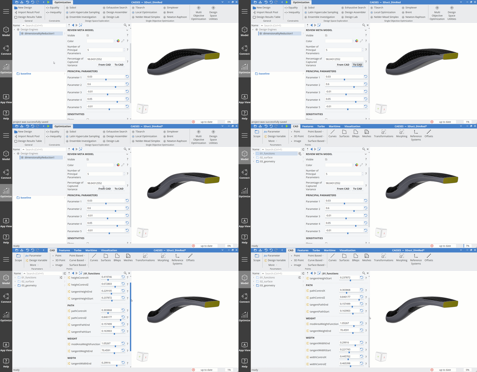
If you open the Design Variable overview in the Model workspace again, you can see that all of the Design Variable values changed to approximate the shape defined by the Principal Parameters.
Extend Sample Set and Change Number of Points per Sample
If the back-transformation returns inaccurate results, it may help to extend the sample set and change the number of points per sample.
- Click on Extend Setup.
- Set the Additional Samples to
100. - Set the Number of Points per Sample to
700. - Press the green play icon to run the Design Engine for the additional 100 samples, that will be added to the sample set.

Exploration Based on Principal Parameters
- Pick the Sobol algorithm from the Design Space Exploration category of the ribbon (in the Optimize workspace > Optimization tab).
Note that the Sobol now shows another category called Dimensionality Reduction.
- Choose dimensionalityReduction1 from the drop-down menu of the Dimensionality Reduction category in sobol1
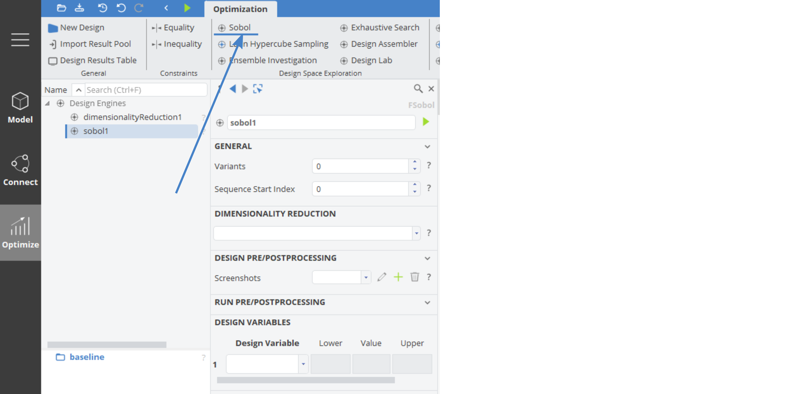
After you set the dimensionality reduction in the Sobol, the Principal Parameter field becomes visible in the Object Editor of the sobol1.
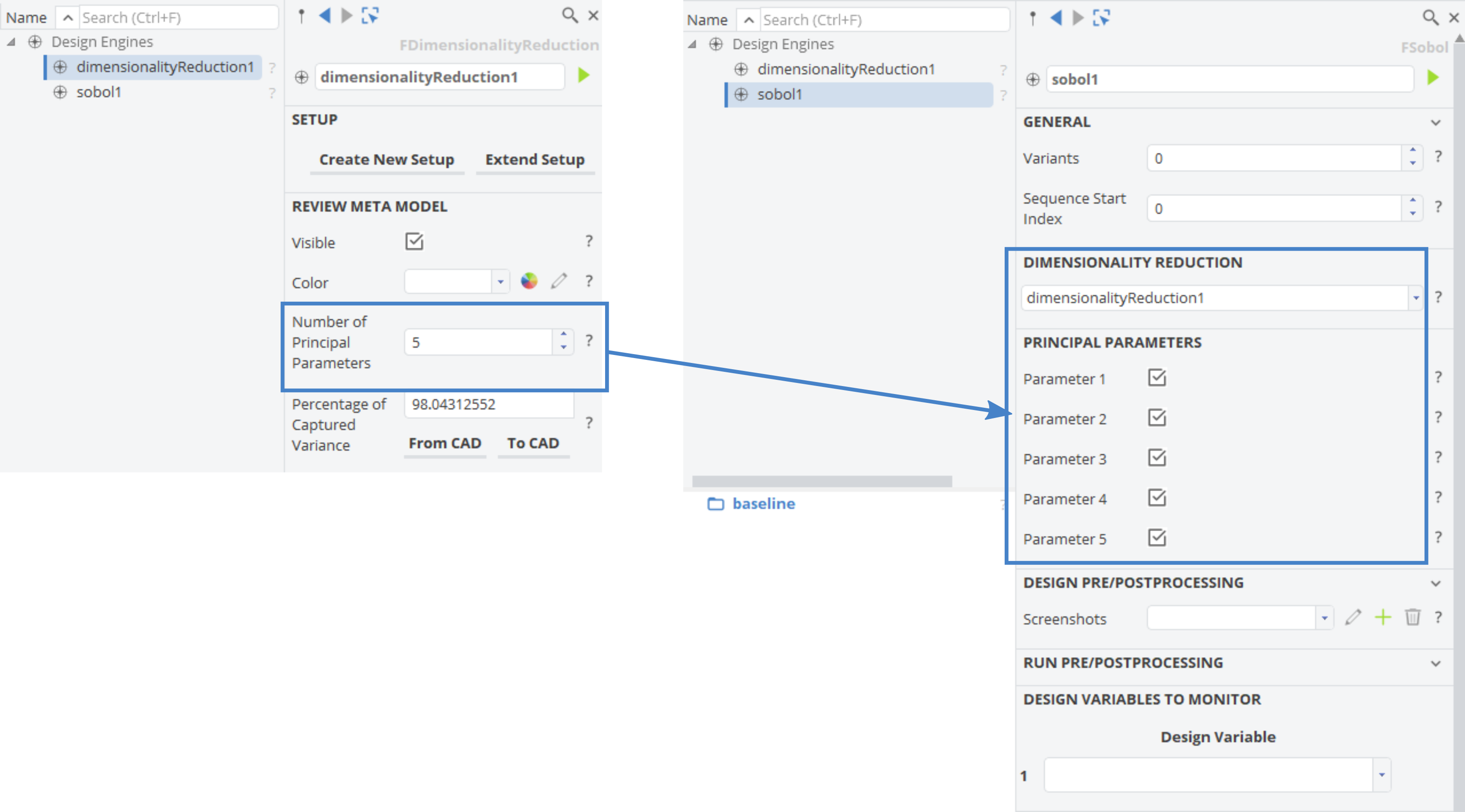
At the bottom of the Sobol setup you can set Design Variables. These Design Variables will only be monitored and appear in the Design Result Table. The Principal Parameters define the new variant shapes. Therefore the Design Variable values depend on the Principal Parameter settings (set by the Sobol) and the back-transformation.
- Set a few Design Variables in the Design Variables fields.
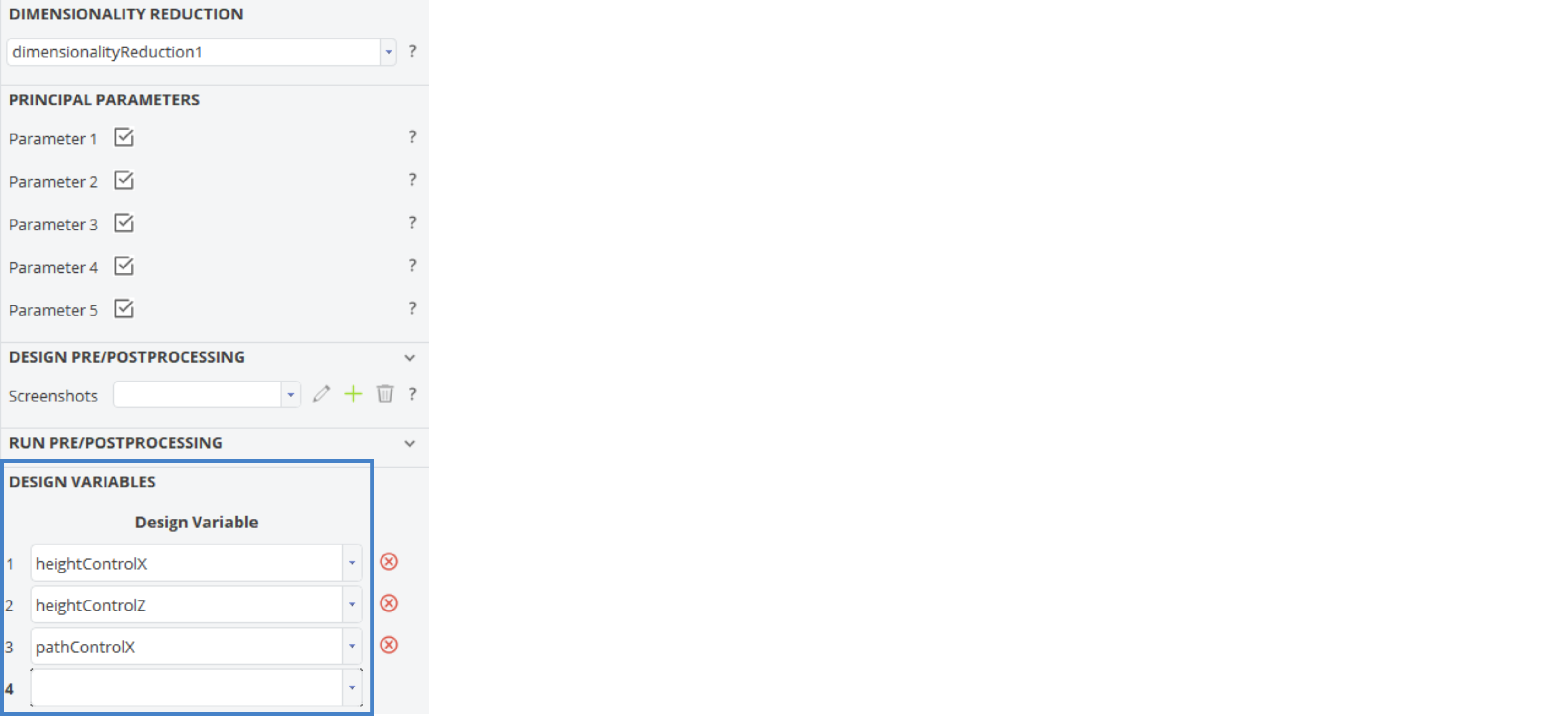
- Add a Screenshot Collection by clicking the green + icon next to the Screenshots field.
Let's run the geometry variant creation in the dimensionality reduced design space with five Principal Parameters now.
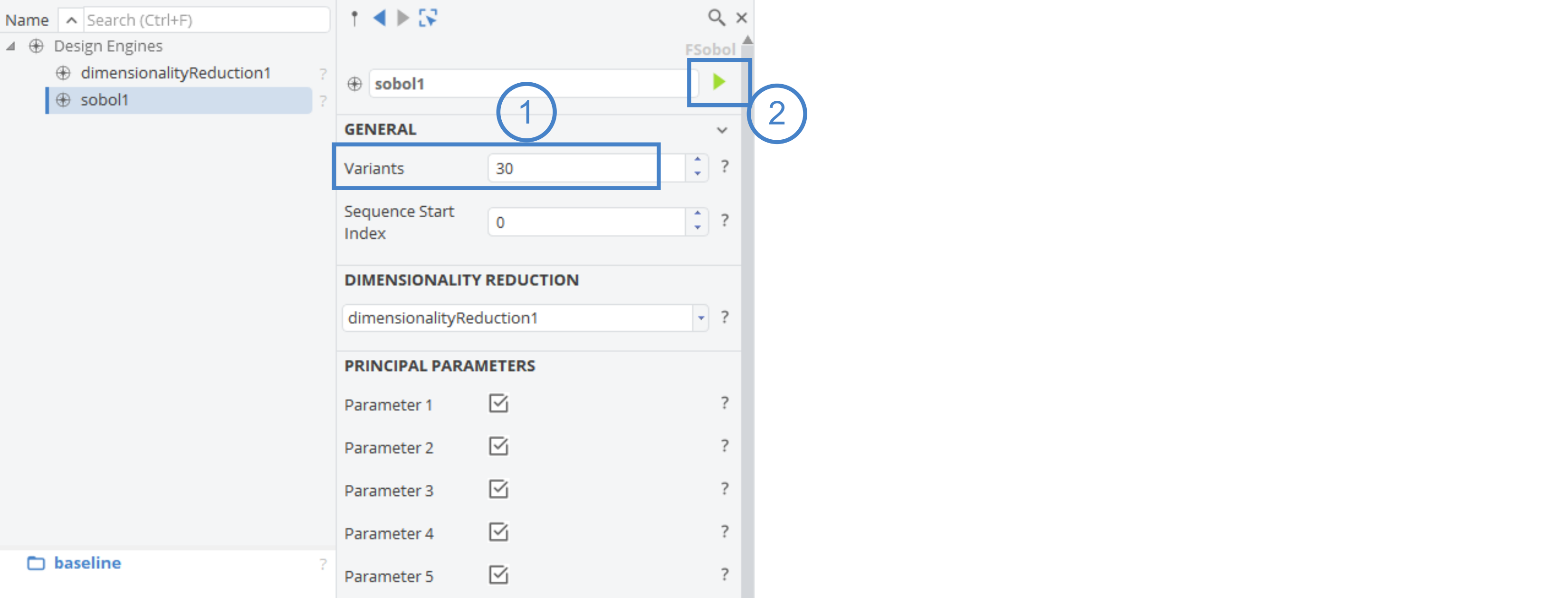
- Set the number of Variants to
30. - Click the Run button to start the geometry variant creation with the Sobol based on the first five Principal Parameters.
Design Result Table
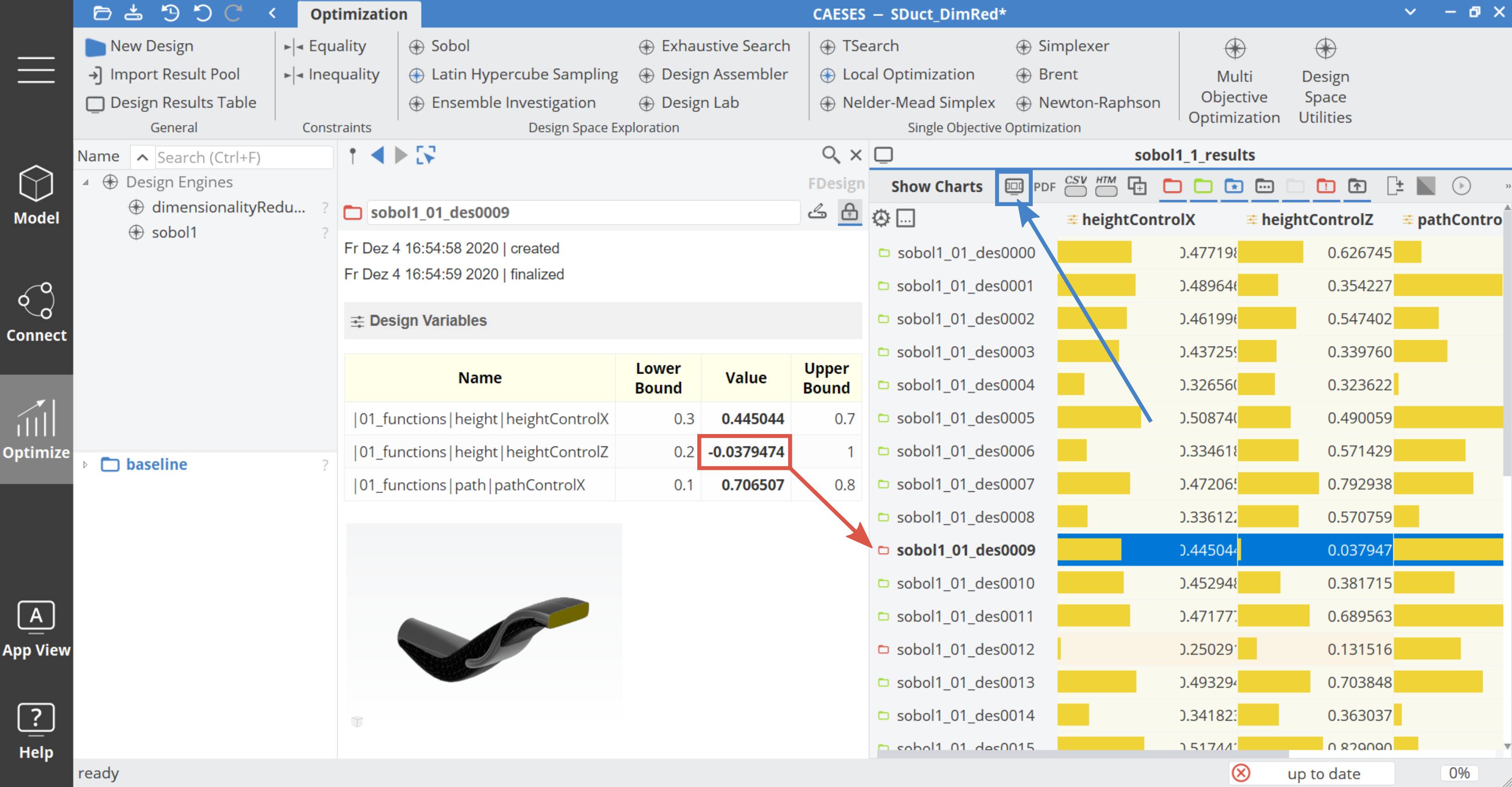
The Design Result Table appears in the Central Window after the Sobol run is finished. The Design Variables we set as Design Variables in the Sobol setup are displayed here. Note that some designs show a red icon, which indicates violated designs. In this case the back-transformation from the Principal Parameters to the nearest approximation of the original Design Variable values has returned values, that lay outside the upper or lower bound of the original Design Variable definition.
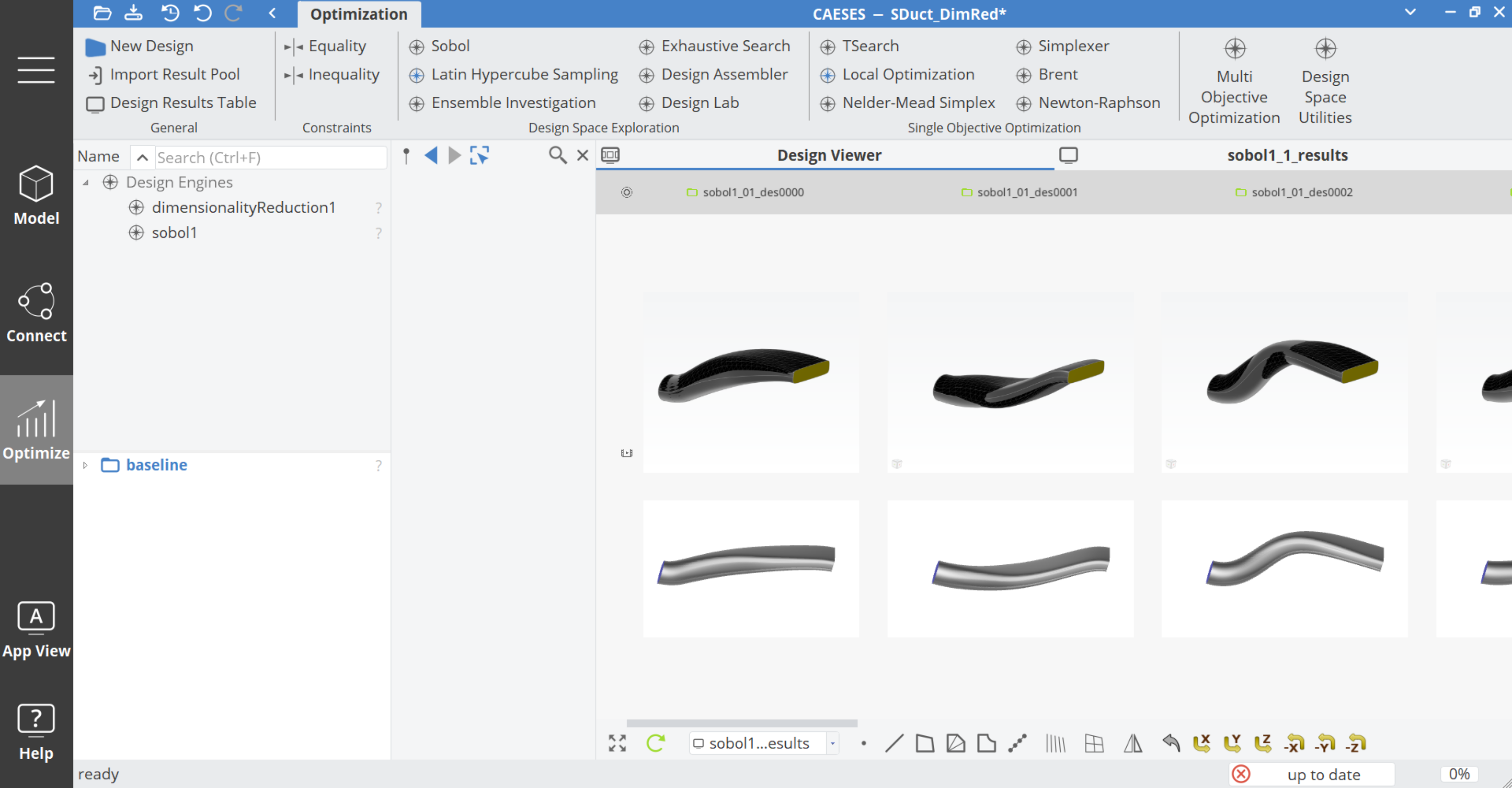
- Click on the Design Viewer icon above the Design Result Table.
A screenshot of every design should be visible now. Take a look at all of the different variants that were created. You can see the black shape, which is what the meta model, defined by the Principal Parameters, looks like. Also, the back-transformed grey BRep model is seen. This also gives us an indication of how well the back-transformation could be performed for the each Principal Parameter setting. Since the back-transformation is non-trivial the back-transformed designs (grey) deviate from the meta model shape (black).
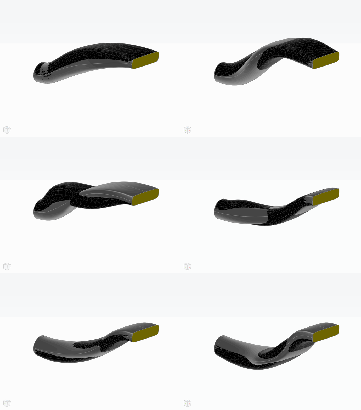
This tutorial showed an example of how a dimensionality reduction could be set up on an S-Duct model. We were able to reduce the original 14 design variables to five Principal Parameters while retaining 98% of the model's variability. Using this method in an optimization algorithm, like the T-Search, can save several simulations and speed-up the optimization process and therefore save significant computational resources.
CAESES Project File
If you want to take a look at the finalized model you can find the resulting CAESES project file s-duct-dim-red-pca.cdb here: