Dakota - Using Advanced Optimization Strategies in CAESES
Besides the standard sampling and optimization methods of CAESES, you can also run additional advanced optimization strategies such as response-surface based methods (RSM). Response surfaces are surrogate models of a real engineering problem, and by carefully generating and using them you can save tremendous computational time. The mathematical methods behind response surfaces can be quite complex, while using them in CAESES is easy. There are also further strategies available such as multi-start methods which run local optimizations from different starting points simultaneously – again very easy to use with a single click.
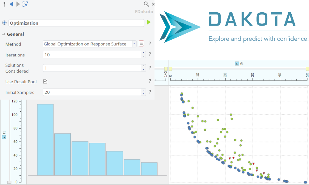
CAESES plugs in these new methods and advanced strategies by wrapping Dakota, the optimization toolkit from Sandia National Laboratories. Users of the AdvancedOpt add-on of CAESES get new design engines in the Optimize workspace where you can choose between pre-configured strategies. This add-on also enables users to do post-processing with handy and beautiful 2D charts.
Dakota based optimization strategies can be distinguished by a blue icon  .
.

Experienced Dakota users can also define and use their own Dakota input files in CAESES, and fully customize the graphical user interface (i.e. customizing the visible design engine input attributes for each method). With this customization possibility, a huge variety of state-of-the-art numerical methods can be immediately used for comprehensive investigation of almost any engineering application.
This tutorial gives a brief overview about how to run these additional optimization strategies in CAESES.
Getting Started
The AdvancedOpt add-on of CAESES comes with a set of pre-configured algorithms that can be readily used. The following steps outline how you can run these methods from within your CAESES project:
- In the Optimize workspace choose a Dakota design engine (blue icon) depending on your optimization problem (a first Design Space Exploration, a Single Objective Optimization or a Multi-Objective Optimization).
- Select one of the pre-configured methods. These methods are explained in more detail on the next pages.
- Set a good name for your design engine, e.g. “Optimization”, “DoE” (Design of Experiments), “Study”, ...
- Configure your design variables, evaluations and constraints as usual.
- Run the design engine.
Pre-configured Methods
The pre-configured methods complement the existing optimization strategies of CAESES. Here is a brief overview of them:
Sampling
This method is a good starting point for many tasks and uses a Latin Hypercube Sampling. Suitable for simple parameter studies and for finding correlations and trends. These randomly-generated designs can be recycled for building up a response surface, see Global Optimization on Response Surface below.
Local Optimization
Gradient-free local optimization strategy. Recommended method to further optimize an existing good design.
Local Optimization Multi-Start
This strategy allows you to run several local optimizations from different starting points at the same time. The starting points are randomly generated. For each local search, a gradient-free strategy is applied.
Global Optimization
Single- / Multi-Objective Genetic Algorithm (MOGA): It can be used for global optimization tasks.
Genetic algorithms need many evaluations. This makes this method suitable only for problems where the evaluation (analysis) is not too expensive. The initial population size as well as the number of generations can be set by the user.
Global Optimization on Response Surface
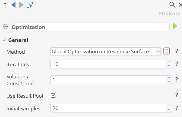
In this method, a MOGA is conducted on a response surface that is iteratively built-up. For the initial response surface, data from a previous run (e.g. a sensitivity analysis) can be considered as well. The best designs of each MOGA run get evaluated and are added to the response surface. This updates and improves the response surface model in each iteration. With this approach, the method tries to reduce the number of expensive evaluations such as CFD runs. The global optimization on a response surface is suitable for single- and multi-objective problems. The Solutions Considered define the maximum number of optimal solutions to be considered after each optimization on the response surface i.e. picked from the Pareto Frontier. Choose as much as possible for more variety with regards to your simulation capabilities or resources. For a single-objective problem only 1 solution is picked and evaluated. All solutions are evaluated after each iteration which typically is a run with your external simulation code. Example: If 10 Pareto designs are found and you consider 2 solutions of it you will have 2 simulation runs per iteration.
Best Practices
There is no optimization method that can be recommended as THE solution for each engineering problem. However, here are some best practices that can guide you in selecting the right algorithm:
Step 1 | Sensitivity Analysis with Sampling
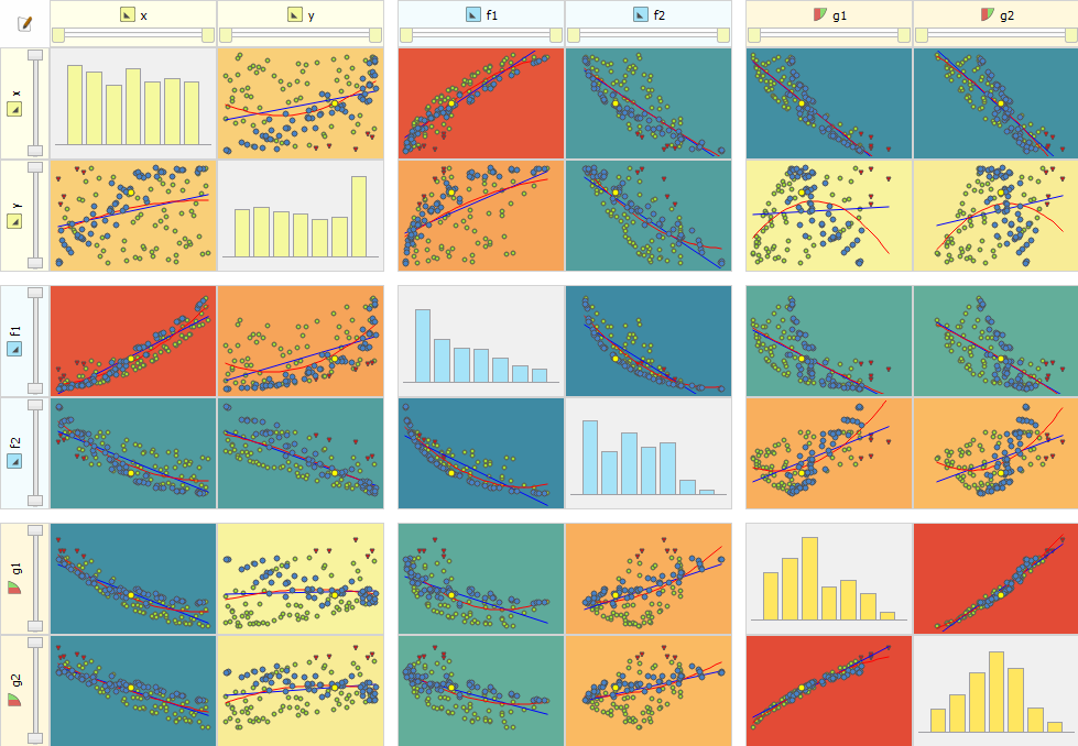
As a starting point, run a Sampling as a sensitivity analysis to get a better understanding of your engineering problem. Check the 2D charts for correlations (colored by red and blue, plus regression curves), and find out which variables you can omit in the next step. The lower the number of variables, the less computational time you will have during optimizations.
Step 2 | Check the Response-Surface Based Optimization
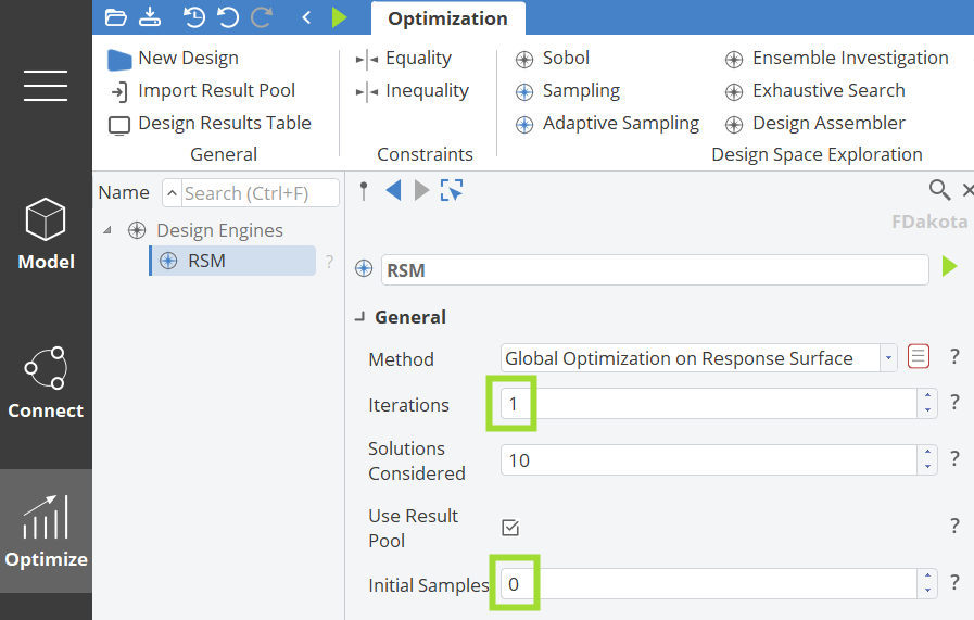
You can try out whether a response-surface based optimization is suitable for your problem. Use a low number of iterations in the first stage by setting the attribute Iterations to 1, 2 or 3.
The input argument Solutions Considered defines how many designs from the Pareto frontier are picked and evaluated (e.g. 10 corresponds to 10 CFD evaluations in each iteration ).
Check the generated designs in the design table i.e. whether they improve and head into the right direction. If it looks promising, continue with a higher number of iterations (e.g. 10).
You can also recycle the previous design results by selecting them as result pool input in the next run. If you set Initial Samples to 0, then no sampling takes place for building the initial response surface. Instead, you can choose the designs from the previous sensitivity analysis (or from any other run). If you set a number that is non-zero, a Latin Hypercube Sampling is triggered internally to create samples that are used for the response surface.
Usually, the number of initial samples needs to be ~5 times the number of design variables.
Alternative: Multi-Start Local Optimization
If the response surface method seems to fail for your task, then you can try to run gradient-free local searches in your domain. The multi-start strategy allows you to run these local optimizations from several different starting points. You can start with a lower number of maximum evaluations to observe trends first.

Improving Good Designs
Suitable design candidates e.g. from a sensitivity analysis can also be further fine-tuned by selecting a single local optimization for this specific design. Here is a short guide how to do this:
- Create a manual design of the promising candidate: Activate the promising design by double-clicking on the design in the design tree. Then, choose New Design in the Optimize workspace to create a new design based on an existing design.
- Select the existing Dakota design engine and create another one. This automatically takes over the design variable settings.
- Choose
Local Optimizationand run the engine with the current design variable settings (i.e. the ones from the promising candidate).

More Information
The brief summary from the previous sections does not cover all the methods’ details. How can you find out more?
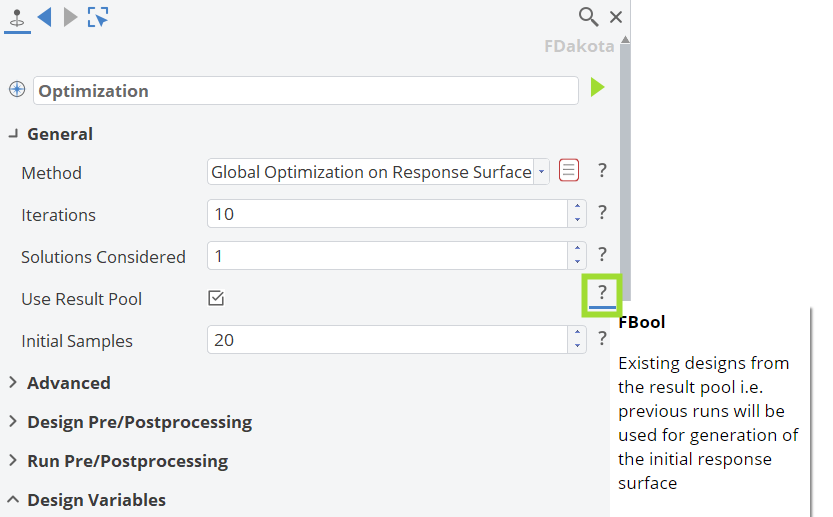
- Click on the help icon (“?”) for more information about the input arguments.
- Click on the template icon in order to take a look at the input file that is used for Dakota:
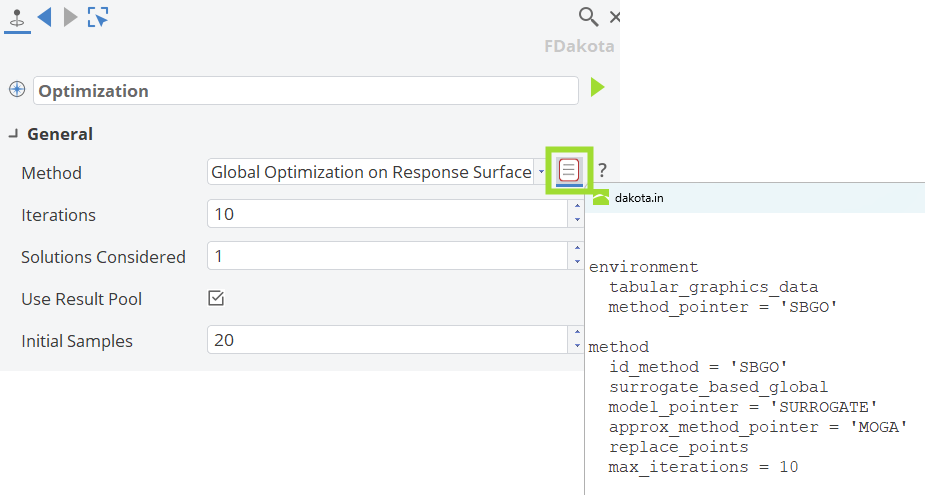
-
Check out the Dakota user’s manual that is also shipped with CAESES. See the installation folder
C:\Program Files\CAESES\etc\integration\dakotawhere you’ll find the PDF document. -
And finally, we recommend to check out the Dakota website if you would like to modify the existing pre-configured methods or if you want to set up your own methods. Take a look at the Custom Templates section for more information.
Charts
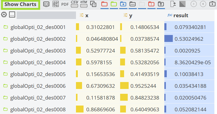
All design engines – including the Dakota engine – generate interactive 2D charts if the AdvancedOpt add-on is licensed. The charts help you understand your results and support you e.g. in finding the most relevant variables as well as picking the best designs e.g. from a Pareto Front.
- You can access them at the top of the result table.
Correlations
For a sensitivity analysis, the red colored fields indicate a positive correlation. If the variable value increases, the objective will increase as well. Blue-colored fields indicate a negative correlation. You can configure the charts by clicking on the upper left edit icon.
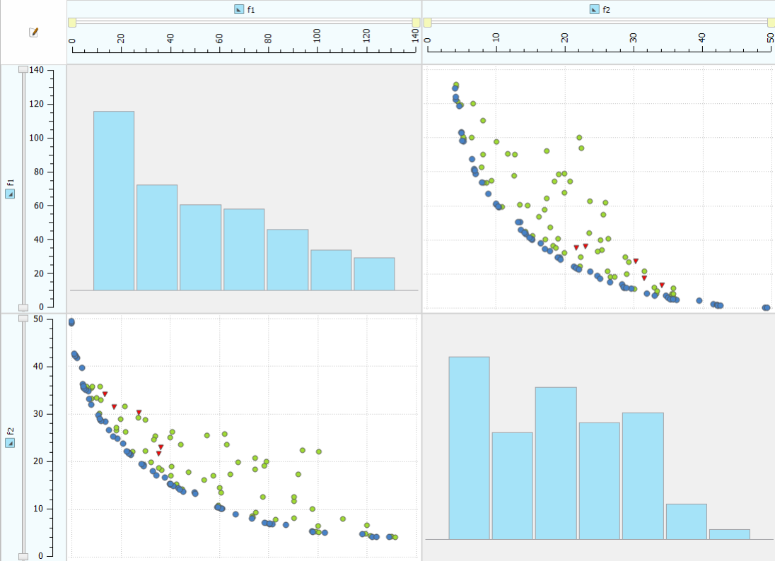
Pareto Front (Multi-Objective Optimization)
A Multi-objective optimization can be started by choosing the Multi-Objective Optimization category > Response Surface Optimization that allows the setting of 2 competing evaluations (objectives). In CAESES, the best designs receive a special blue-colored icon (with a star on it). In addition, the best designs are colored blue in the 2D charts. This makes it easy to pick them e.g. from a Pareto Front where you have several competing objectives. Valid designs receive a green dot, while the red triangles are designs that violate some of the constraints. As an option, you can use the controls on the left and on the top to set the boundaries (limits) of what is shown.
Custom Templates
You can also set up your own Dakota input files, to make use of the entire Dakota method set, and hand it over to the Dakota design engine.
- As a start, check out the pre-configured input files that are presented in this tutorial. See the installation folder
C:\Program Files\CAESES\etc\integration\dakota. There you will find these files (*.in) for Dakota that are used by CAESES. Make a copy of one of them, store them somewhere else and start modifying it. - For the method attribute, select “Custom” and choose your input file.
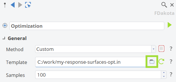
CAESES Keywords
In the CAESES installation folder in etc > integration > dakota folder, you will also find a file called template_definitions.txt. This gives you an overview of the CAESES keywords that you need to involve for setting up your own template. For instance, CAESES automatically writes the number of objectives into the Dakota input file, for which a CAESES keyword eval_count_objective needs to be used.
CAESES keywords for custom Dakota template definition
GENERAL
#name name to be displayed in template box
#docu
documentation to be displayed as tooltip
use html formatting and do not forget #!docu to end the documentation section
#!docu
If a single objective algorithm is used, you can add the
#singleobjective
flag to prevent the algorithm from running when multiple objectives are set.
ATTRIBUTES
Documentation has to be inside of "" if it contains colons.
<key, type (unsigned/int/double/bool/key/enum(val1@DropdownName1@HoverDocu1; ...; valN@DropdownNameN@HoverDocuN)) [, default value, attribute name, docu, category, weight(int), always show(bool)=true, refreshes editor (bool)=false, is hidden command(bool)=false, should be written command(bool)=true]>
if key starts with !, only the value will be written.
DESIGN VARIABLES
number of design variables:
[dv_count]
initial values of design variables:
[dv_initial_values]
lower bounds of design variables:
[dv_lower_bounds]
upper bounds of design variables:
[dv_upper_bounds]
names of design variables:
[dv_names]
DESIGN VARIABLES (discrete design set): CURRENTLY USED FOR INACTIVE DESIGN VARIABLES WITHIN RESPONSE SURFACE TECHNIQUES
number of design variables:
[dv_dds_count]
initial values of design variables:
[dv_dds_initial_values]
names of design variables:
[dv_dds_names]
IMPORTANT
Keep the following order of keywords inside your template definition:
- objectives
- evaluations
- inequality constraints
- equality constraints
evaluations:
total number of objectives + evaluations:
[eval_count_all]
number of objectives:
[eval_count_objective]
number of evaluations
[eval_count_evaluation]
names of objectives + evaluations:
[eval_names_all]
names of objectives:
[eval_names_objective]
names of evaluations:
[eval_names_evaluation]
constraints:
total number of inequality + equality constraints:
[constr_count_all]
total number of equality constraints:
[constr_count_equality]
total number of inequality constraints:
[constr_count_inequality]
names of inequality + equality constraints:
[constr_names_all]
names of equality constraints:
[constr_names_equality]
names of inequality constraints:
[constr_names_inequality]
Example Code for Custom Dakota Template
#name Global Optimization

#docu
Global optimization using the genetic algorithm MOGA. It can be used for global optimization tasks. Note that, in general, genetic algorithms need many evaluations. This makes this method suitable only for problems where the evaluation is not too expensive.
#!docu

method
  moga
  output debug
  seed = 12345
  crossover_type shuffle_random
  num_offspring = 2 num_parents = 2
  crossover_rate = 0.8
  mutation_type replace_uniform
  mutation_rate = 0.1
  fitness_type domination_count
  replacement_type below_limit = 6
  shrinkage_percentage = 0.9
  niching_type distance 0.15
  postprocessor_type
  orthogonal_distance 0.05
  convergence_type metric_tracker
  percent_change = 0.05 num_generations = 10
  <max_function_evaluations, unsigned, 300, Samples, set maximum number of function evaluations, General, 0>

variables
  continuous_design = [dv_count]
  initial_point [dv_initial_values]
  lower_bounds [dv_lower_bounds]
  upper_bounds [dv_upper_bounds]
  descriptors [dv_names]

responses
  objective_functions = [eval_count_objective]
  nonlinear_inequality_constraints = [constr_count_inequality]
  nonlinear_equality_constraints = [constr_count_equality]
  no_gradients
  no_hessians

[interface]
  asynchronous
  <evaluation_concurrency, unsigned, 8, Maximum Number of Pending Designs, maximum number of pending i.e. parallel running designs, General, 4, false>
RESPONSE SURFACES
You can generate response surfaces by re-using existing data.
Checks for string model.dat in template file and writes yellow bin to be used as sample points by Dakota.
Example:
<reuse_samples all points_file = 'model.dat', key, true, Use Result Pool, Use Result Pool for Response Surface Generation, response surface creation, 0, true>
Customizing the CAESES GUI
When you write your own method setup for Dakota, you can also configure the user interface. This means that you can control what is transferred to the interface and what’s hidden (e.g. when the default value should not be changed). Finally, you can add documentation to a Dakota attribute. Here is a snippet where the Dakota keyword samples has been wrapped by the CAESES user interface:
method
sampling
sample_type lhs
<samples, unsigned, 100, Samples, number of samples>
seed = 12345