Surfaces

CAESES provides a set of different parametric surfaces s(u,v) that can be found in the menu

• Model > CAD > Surfaces.

This section gives you a brief introduction the most important surface know-how. Check the help-icons of the properties to learn about each individual input of the different surfaces.

Surface Types

The different surface types are grouped by the inputs to create the surface. These are:

• Point Based
• Curve Based
• Surface Based

FSurface

The FSurface is the basic type for surfaces. Every other surface type is in the hierarchy below this type. The functionality of this surface is to provide a Creation Method, which can be dynamically switched, which is why it also called a "dynamic type".

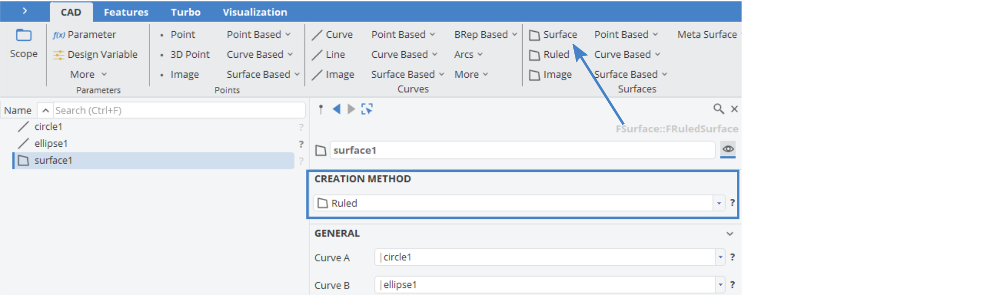
When the Creation Method is switched, all dependencies to this surface will be preserved.

Surface Properties

Surface Domain

Similar to the curves in CAESES, all surfaces are defined through a parameter space, (U,V). It is defined in the global xy-plane in the interval [0,1] x [0,1].

This 2D domain is mapped into the 3D space to create the surface. The following picture shows a 3D surface where the orientation is visualized, along with the UV-coordinates:

tip

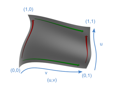
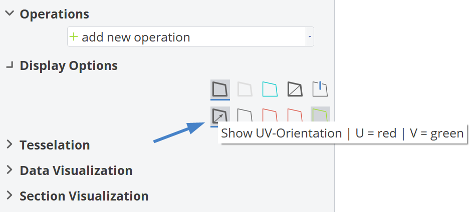
In the Object Editor of the GUI, under Display Options, you can show UV orientation: U is displayed in red and V in green

Boundary Curves

When you activate the subselection mode and hover over the boundary of a surface, a surface curve is indicated which can be used as a standard curve. For instance, you can put such a curve into an image curve for further processing. The start and end positions are also readily available (e.g. surface:edge1:start).

There are always two differently oriented surface curves offered, depending on whether you hover the mouse cursor over the beginning or over the end of the boundary. This is a convenient mechanism to have both curve orientations available.

tip

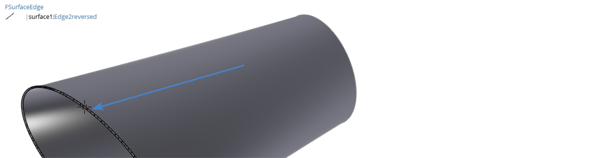
For adjacent surfaces, make sure that you move the mouse cursor from within the surface (from which you want to get the surface curve) into the direction of the boundary. Otherwise, it might detect the surface curve from the adjacent surface.

Surface Positions

In order to calculate and receive a surface position of a surface with name "s", use the position command:

s.getPos(u,v)

where "u" and "v" can be a value in the range [0,1]. This returns a vector.

Create a Point on a Surface

When you select a surface and create a 3D point (while still having the surface selected), it will automatically create the point on the surface using the position command.

Surface Orientation

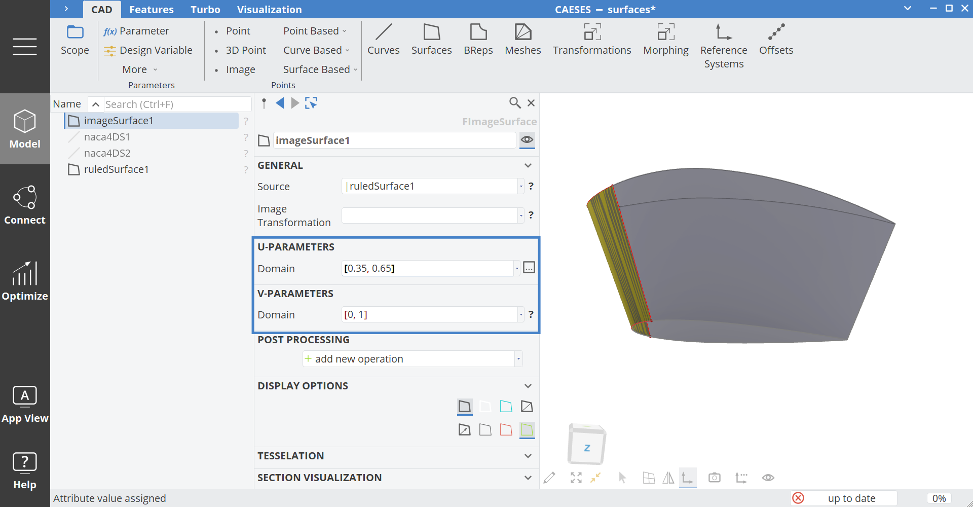
In order to change the UV-orientation of a surface, use an image surface which you find in the menu

Model > CAD > Surfaces > Surface Based > Image Surface.

The image surface has two domain intervals, one for the U- and one for the V-domain, respectively. Both can by changed by the user. By default these domains are set to the entire range, i.e., [0,1]. You can change it e.g. to [0.25,0.75] in order to receive only a part of the source surface.

This also allows you to swap domains (2nd level option of general category) or to reverse domains by reversing the U- or V-interval from [0,1] to [1,0].

Reversing can be useful to correct orientations in a parametric model or to make sure that all triangle normals point either inwards or outwards in the context of STL data generation.

Display Options

Note that surfaces also have a set of display options to visualize more information. Examples are the render resolution, color, domain orientation, curvature visualization. Not all these options are shown in the user interface by default - just click on the display options category to expand 2nd level options.

Surface Curvature

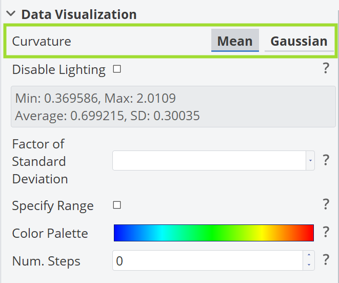
CAESES can illustrate two types of curvature under Data Visualization: Mean curvature and Gaussian curvature. The difference lies in the automatically generated range, which is reflected in the boundaries of the color palette.

Below is a surface colored by curvature values:

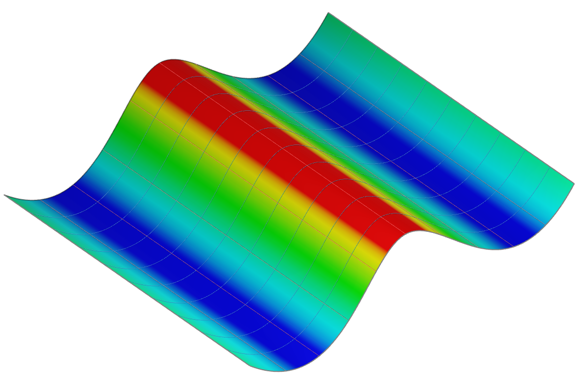
• Positive curvature: surface bends in the same direction (e.g. a sphere).
• Zero curvature: surface is flat or cylindrical (e.g. a plane or a cylinder).
• Negative curvature: surface bends in opposite directions (e.g. a saddle).

Section Visualization

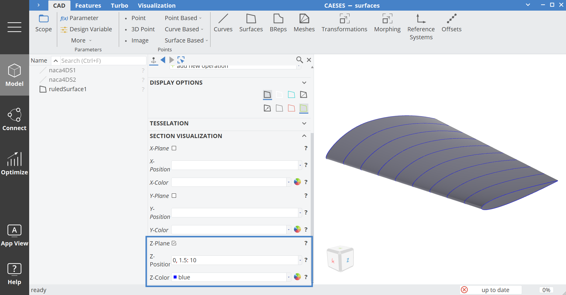
There is also the option to visualize 2D sections on the surface. These sections can be based on a series of values and a principal axis. There are filters at the 3D view to exclusively show sections, or to hide all of them. An example is the visualization of ship hull sections in longitudinal (x) direction and the visualization of wing cross-sections etc.

Create from a Selection

If you have a selection while creating a surface, it will take into account the selection and tries to call a suitable creation command. For instance, select two 3D curves and choose Model > CAD > Surfaces > Curve Based > Ruled.This will automatically set the two curves as input for the new ruled surface.

Standard Surfaces

There is a set of standard surfaces available in CAESES that you can find in the surface menu:

• NURBS Surface
• Coons Patch
• Lofted Surface
• Ruled Surface
• Surface of Revolution

Simply create them through the menu and set the properties.

NURBS Surfaces

If you select NURBS surfaces (e.g. from imported data), there are also buttons at the top of the CAESES GUI to directly manipulate the surface orientation. So, in this case there is no need for an additional image surface.

Coons Patch

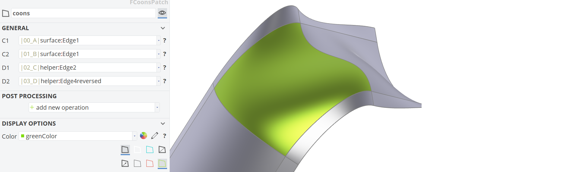
The coons patch allows you to create a surface in between of a set of 4 boundary curves. You can find it in the menu

Derivative Information

If you want to involve derivative information from adjacent surfaces, you need to provide surface curves. From these surface curves, CAESES computes the tangential information for a smooth transition.

Lofted Surface

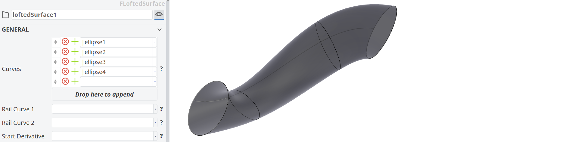
Use the lofted surface if you have a set of cross-sections that you want to interpolate in order to create a surface. The cross-sections need to be sorted running from the start to the end cross-section, as well as aligned in terms of each cross-section's orientation. You can find it in the menu

• Model > CAD > Surfaces > Curve Based > Lofted.

Rail Curves

You can optionally provide rail curves that guide the surface during the lofting process. Make sure the orientation is correct, i.e., they run from the starting cross-section to the terminating one. All cross-sections need to be connected to the rail curves.

Derivative Information

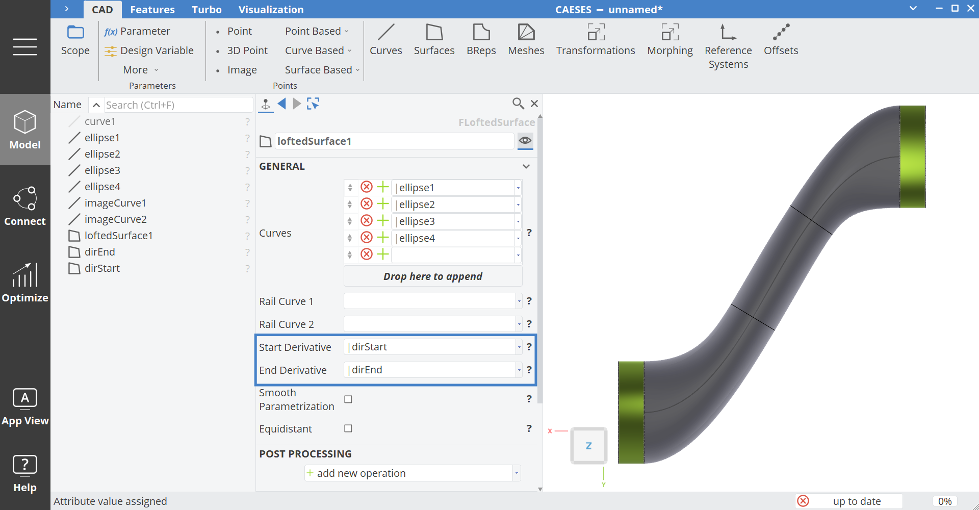
Often you want to control the transition of the lofted surface if adjacent surfaces are connected to it. Here you can simply add these surfaces as a provider for derivative information. This information is then taken into account for the tangential transition while still interpolating the cross-sections.

The following picture shows a lofted surface with 2 cross-sections (which are surface edges in this example), 2 rail curves and derivative information that is simply delivered by the two adjacent (grey-colored) surfaces:

Gordon Surface

The gordon surface type allows you to create a smooth surface based on an input curve mesh. Create it via

• Model > CAD > Surfaces > Curve Based > Gordon Surface.

The input mesh curves must fully intersect, and the parameter values at the intersections must match fairly closely along each row and column of the input curves. Each set of curves (U and V) must be parameterized in the same direction. So, take care of a clean input mesh to make this surface type work correctly.

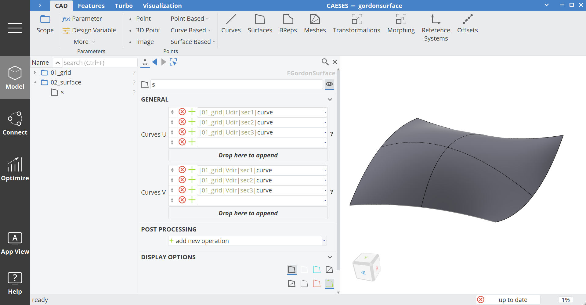
Sweep Surfaces

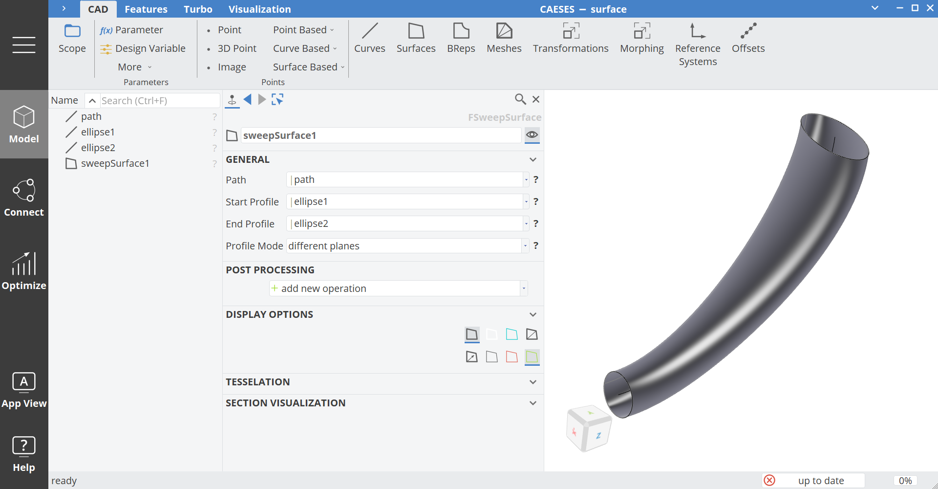
There is an easy-to-use surface type to create a sweep based on either a single or two given 2D contours and a 3D path. You find it in the menu

• Model > CAD > Surfaces > Curve Based > Sweep.

If you need more control and more degrees of freedom during along the whole sweep range, see the meta surface section below.

Meta Surface

The meta surface of CAESES is the most flexible surface type and used in various applications, so that a few comments are dedicated to it in this section. It is highly recommended to first understand how curves and features work before you jump into meta surfaces. You can find it in the menu

• Model > CAD > Surfaces > Meta Surface > Meta Surface.

The meta surface is basically a parametric sweep surface. But instead of only providing a sweep contour for the start (and optionally for the end), you can control the shape distribution during the whole sweep range.

info

You can also understand meta surfaces as lofted or skinned surfaces where the cross-sectional curves are controlled in an efficient way.

The exciting part is that you can define any curve and any sweep direction by using your own custom parameters, for any application. And all of these parameters can be efficiently controlled in 3D space. Efficiency finally means smooth surface shapes with less parameters (free variables in optimizations). This makes it a fully generalized tool for the creation of any kind of 3D surface.

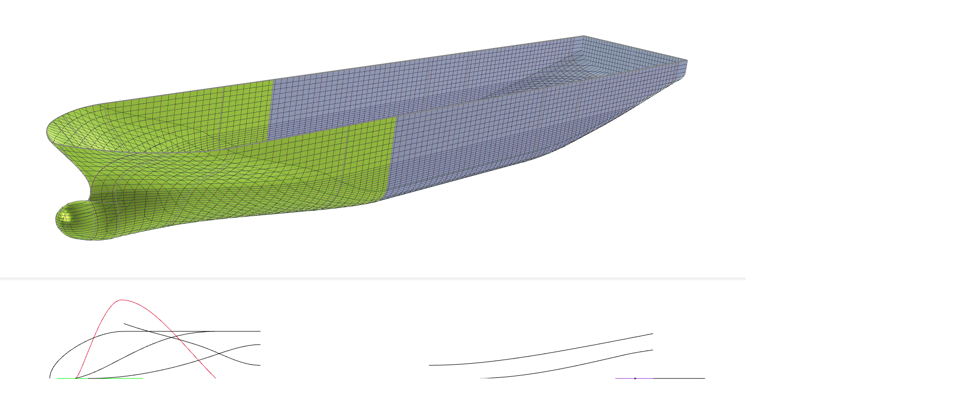
Meta Surface Examples

• Control the displacement and section shapes of ship hulls at each longitudinal x-location.
• Control the blade profile parameters such as camber values and thickness values in span-wise direction (and not only at the hub and tip region). Works for any type of blades, e.g. for fans, propellers, impellers, pumps.
• Control the cross-section area of manifolds, channels, diffusers along the sweep direction.
• Control any custom volute parameters for turbochargers and pumps.
• Control asymmetric piston bowls designs where also the compression volume needs to be kept.
• Control the shape of automotive springs at each location of the wrap.

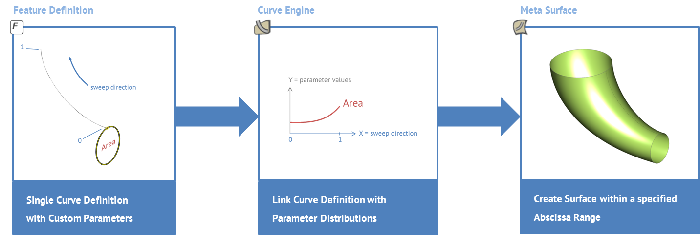
Meta Surface Process

In a first step, you create a feature definition which describes your curve (that you want to sweep). This curve has a set of parameters including the "sweep parameter" that will be used to sweep the curve into the 3D space and to create the surface.

Secondly, you create function graphs for all of your curve parameters. Most often, this is done in the xy-plane, where normalized functions are define, i.e., running in the x-interval [0,1] and in the y-interval [0,1]. The sweep parameter of your definition typically has a linear function, e.g. if it is a curve path parameter there would be a linear function from 0 to 1.

info

The use of functions reduces the number of free variables drastically, and typically creates smooth surface shapes if you also use smooth functions.

As an intermediate step now, create a curve engine (Model>CAD>Surfaces>Meta Surface> Curve Engine) which connects the curve definition to the parameter functions. This engine is now basically able to create your curve at any 3D location according to your function graphs.

tip

Just as a comment: There is even a curve engine command myEngine.getCurve(where) to receive a curve and that you can store in an image curve e.g. for testing purposes. The argument where is an x-abscissa value (between 0 and 1) if you have modeled your functions in the xy-plane.

In the last step you create a meta surface that takes the curve engine and generates the surface. The following picture illustrates the whole process:

Once you have understood this 3-steps-concept

1. Feature definition
2. Curve engine and functions
3. Meta surface

you gain a maximum of flexibility to design any parametric surface in CAESES with highly efficient controls for CAE applications.

Domain Modeling

In the context of sub-surface modeling which can be done manually by yourself in the domain of the surfaces, CAESES offers 3 important curves. You can find them in the curve menu CAD > curves:

• Surface curve
• Intersection curve
• Projection curve.

All these types have domain curves in the 2D UV-space of the surface they are working with. You receive the domain curves by calling the command sc.getDomainCurve() for a curve with the name "sc".

This is useful for advanced sub-surface modeling where you create your own (4-sided) UV-space for custom trimming operations etc. Typically, these curves are stored in image curves, to have them readily accessible in the project setup.

There is a subsurface example in the sample section of the documentation browser which illustrates this kind of UV-modeling.

Note that for general trimming operations the use of the BRep type is recommended. You find BReps in the menu Model > CAD > BReps > BRep, and there is also a separate section "Solids" which describes how to use them.

info

Remember the hierarchy of types in CAESES: The mentioned 3 curve types have the same parent type, FSurfaceCurve, which provides the .getDomainCurve() command. Or in other words, all of these are essentially surface curves.

Static Surfaces

In CAESES, you can create a static version of a Surface.
This is done by first selecting the desired surface or BRep face (using the subselection mode) and then using a Point Based Surface > NURBS or B-Spline to generate a detached surface with input points that match the selected original surface. If your selected surface is a BRep Face, the untrimmed original BRep Face will be represented by the static NURBS surface.

The resulting surface is created with fixed values for:

• Control points
• Knot vector
• (For NURBS) Weights

Since these values are fixed, the geometry is no longer connected to any parameters — it is a purely static representation.

tip

Static geometries can be used as reference models and compared against different variants of a parametric model.

Isophotes (Zebra Stripes)

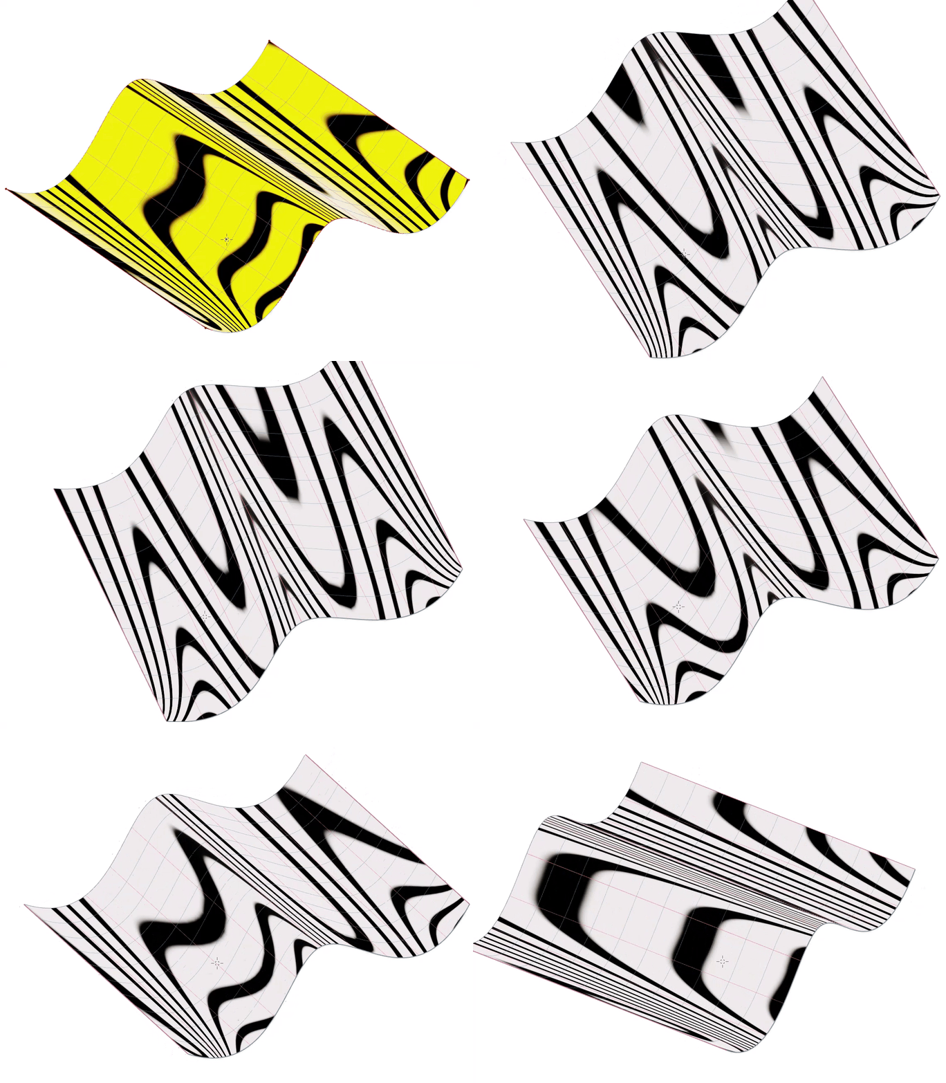
Isophotes, also known as zebra stripes, are a technique for analyzing surface smoothness. They simulate the reflection of stripes on a surface, resembling the appearance of zebra patterns.

In CAESES, isophotes can be enabled in the 3D-View by selecting the pencil icon at the bottom left and enabling the corresponding Isophotes option. The appearance and properties can then be controlled under this section.

Purpose of Isophotes

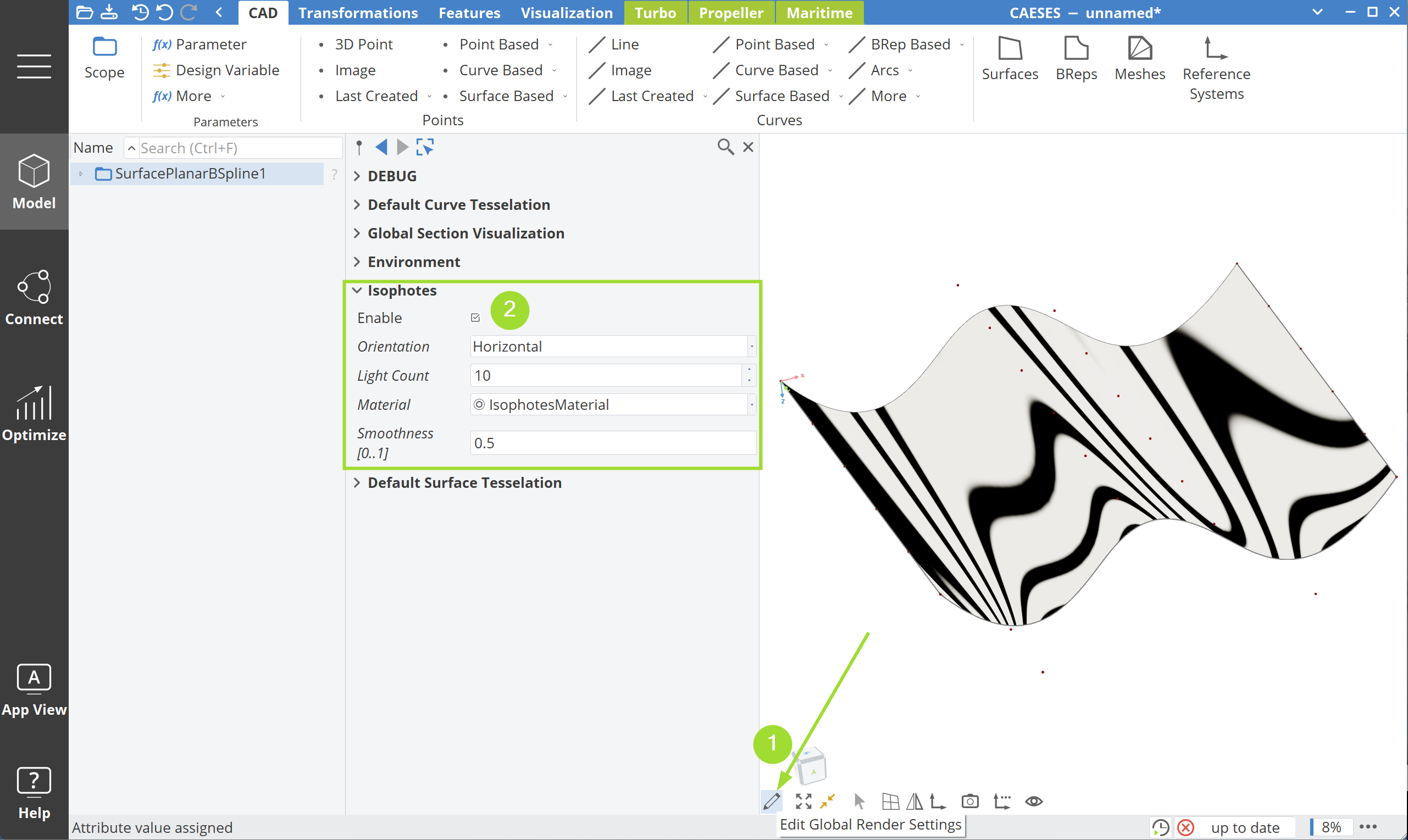
• Identify surface irregularities, such as bumps or discontinuities.
• Ensure smooth transitions between adjacent surface patches.
• Smooth surfaces show evenly flowing stripes, while irregularities cause breaks or distortions in the pattern.