Cylindrical Transformation
The Generic Blade from the previous tutorial maps 2D profiles onto a cylindrical surface. This specific transformation is also separately available in CAESES and can be used in combination with Meta Surfaces. It represents a more generalized way for setting up blade-like surfaces. For instance, some designers have their own nomenclature for radial functions (the Generic Blade uses rake, skew and pitch). Additionally, the Cylindrical Transformation can be used to add basic support geometries to your blade which can then be used for example to define the computational domain for CFD or meshing processes.

The focus of this tutorial is not profile design but understanding the process of setting up a blade with the Cylinder Transformation in CAESES. Therefore, we will create a very simple profile that represents any kind of (complex) profile definition.
Profile
In order to understand the concept of using the Cylinder Transformation entity, we will quickly create a representative profile.
The 2D definition of the profile needs to be given in the global XY-plane. The values along the X-axis will then be interpreted as -coordinates, while the values along the Y-axis will be interpreted as the Z-coordinates of the Cylinder Transformation (see next step Image Curve and Transformation).
-
Create a line via Model workspace > CAD tab > Curves > Line and name it "profile".
-
Set the Start Position to
[-0.5,0,0]. -
Set the End Position to
[0.5,0,0].
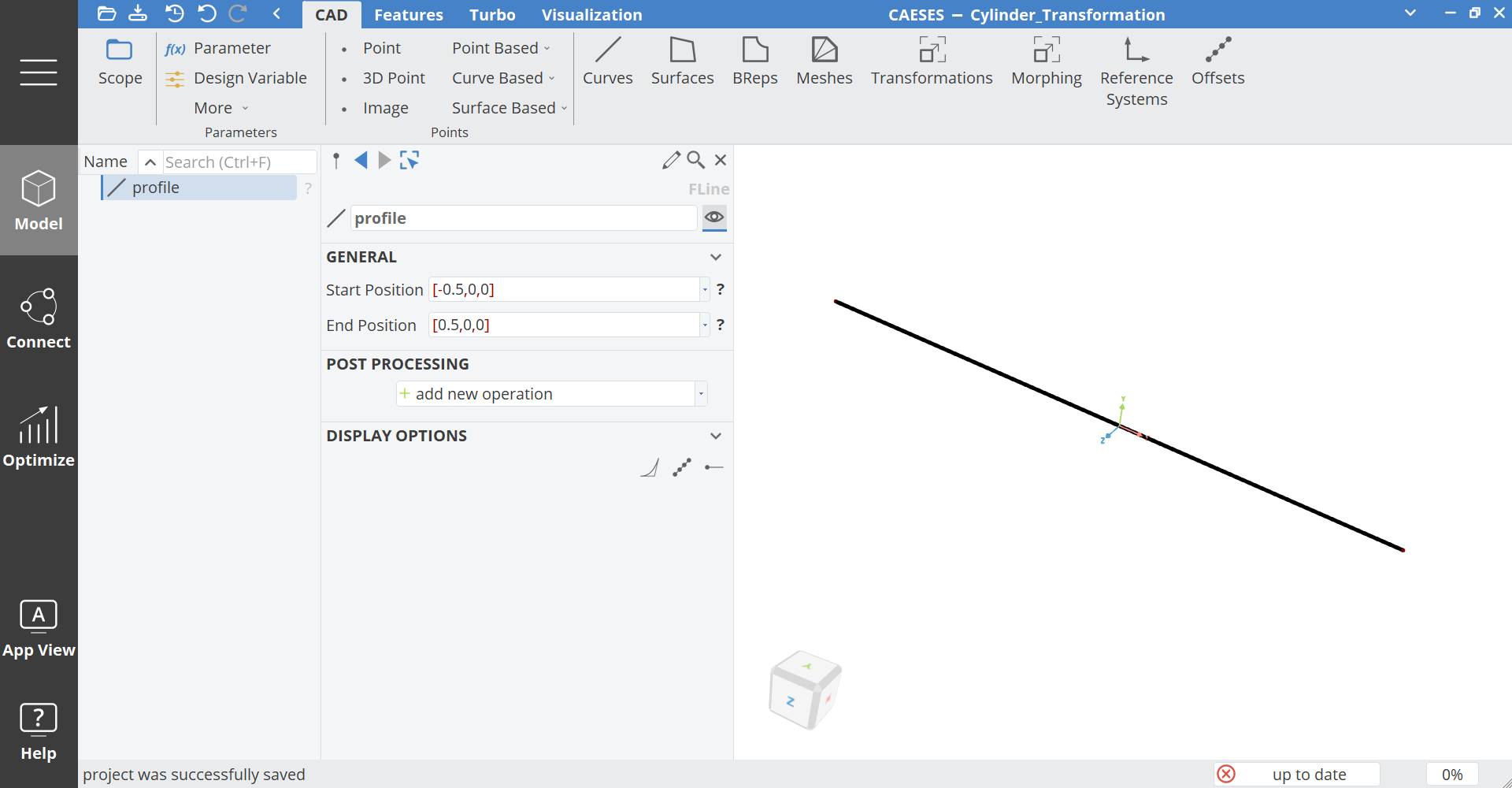
We can also use 3D points (F3DPoint) instead of simple vector data for the positions. When it comes to Meta Surfaces, vectors can accelerate the curve generation process within features:
- Vectors hold only the values while 3D points are managed objects with a set of attributes such as name, scope, color. In our case this is not relevant but for Feature Definitions with many points, this effect sums up and slows down the curve generation process. Therefore, use simple vectors if a point is not necessarily required. It also keeps your project slim.
Image Curve and Transformation
The initial profile will be mapped into 3D space using the Cylinder Transformation:
-
Make sure that the initial curve profile is selected.
-
Create an Image Curve via Model workspace > CAD tab > Curves > Image and name it "profile3D".
-
Create a Cylinder Transformation in the Model > CAD > Transformations > Cylinder.
-
Set the name of the new cylinderTransformation1 object to "transformation."
-
Select the Image Curve profile3D and choose the transformation from the pull-down menu of the attribute Image Transformation
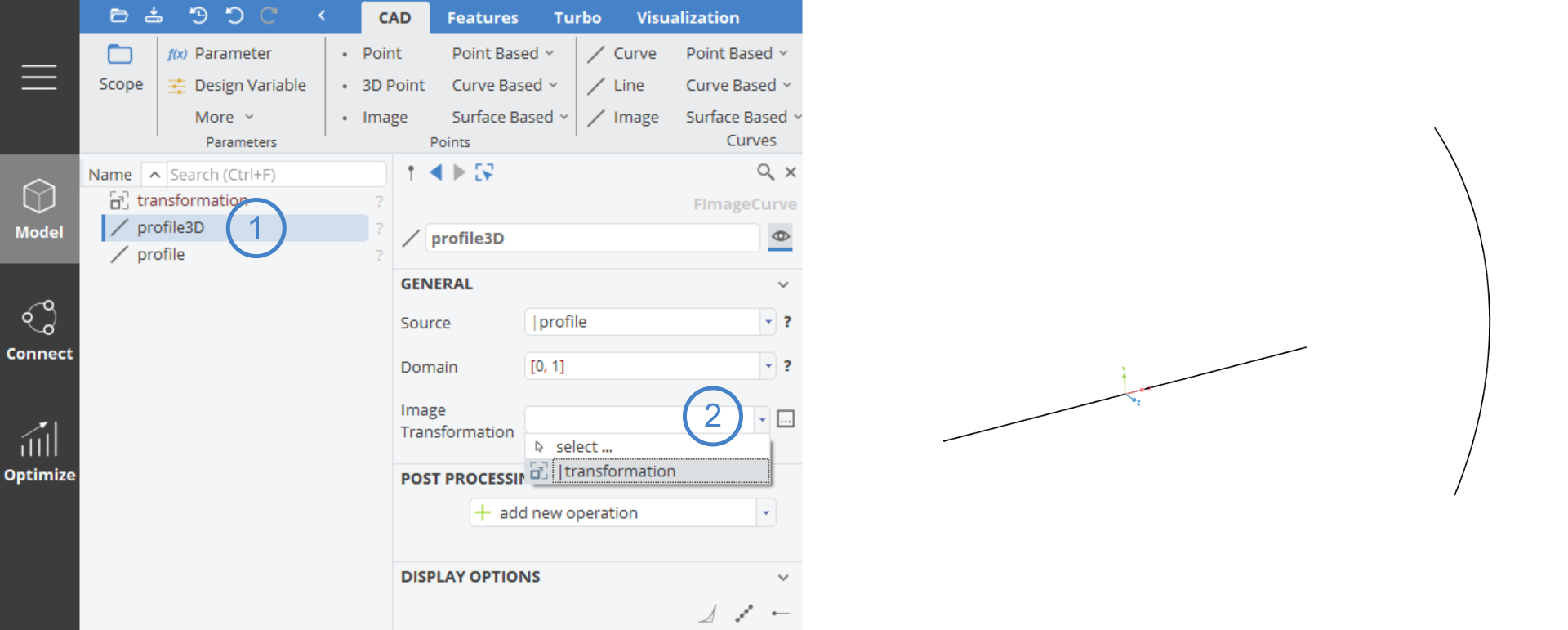
Parameters
You can now change the Radius of transformation and directly see how your profile is mapped into 3D space. In this step, a length and a radius parameter are introduced since these will be the variable values for our upcoming Feature Definition.
-
Mark the value
0.5of the profile's Start Position and create a Parameter via the context menu (right mouse button on the marked value). -
Set the name of the new Parameter to "length".
-
Set the Parameter also for the X-coordinate of the End Position of profile.
-
Divide the expressions by
2so that the parameter controls the length of the total curve (ensure-precedes length at the Start Position). -
Reset the length Parameter value to
1.
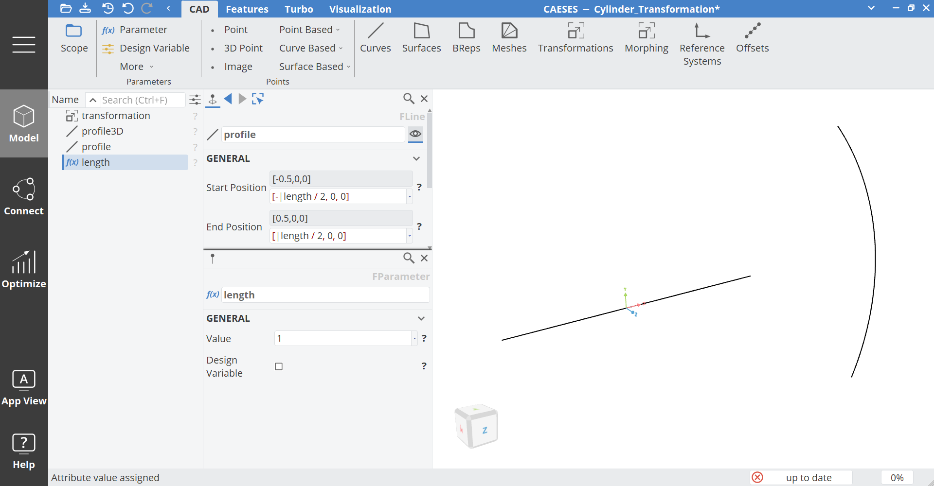
- Create a Parameter for the Radius of transformation via the context menu.
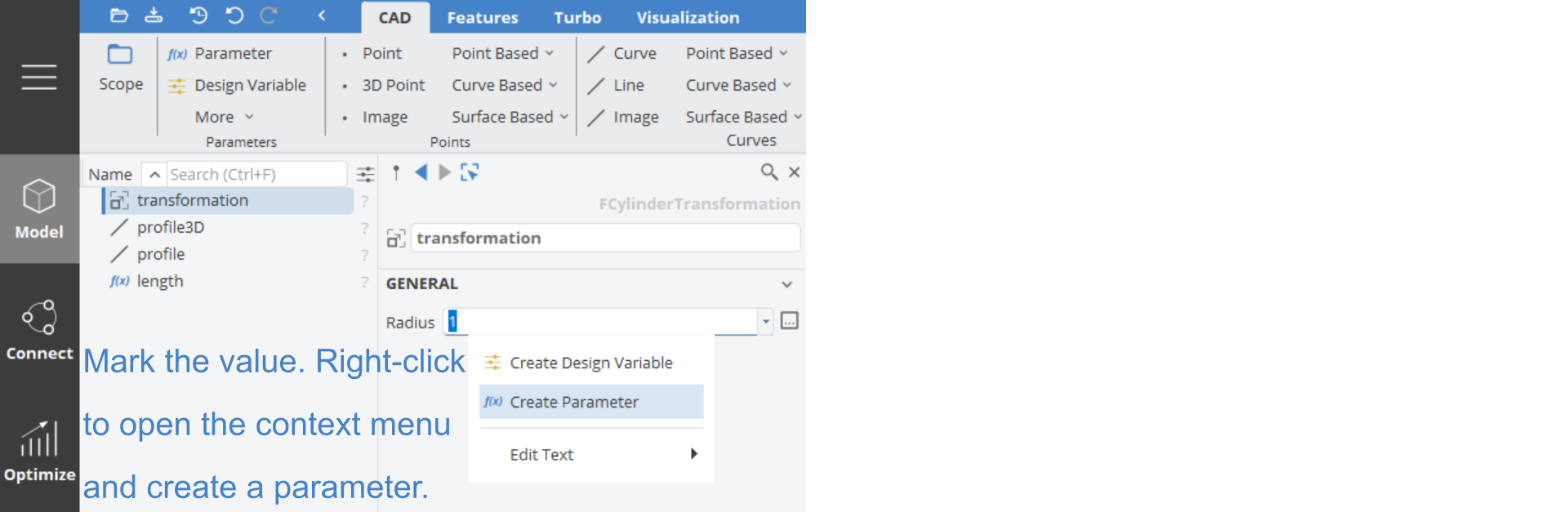
- Set the name of the new Parameter to "radius".
Feature Definition
The curve profile3D is now variable according to its length (length Parameter in the profile) and the radius value (radius Parameter in the transformation). Since we will use a Meta Surface (and a Curve Engine) it requires a curve from a Feature Definition (also see the Meta Surface tutorials).
Let's create the Feature Definition:
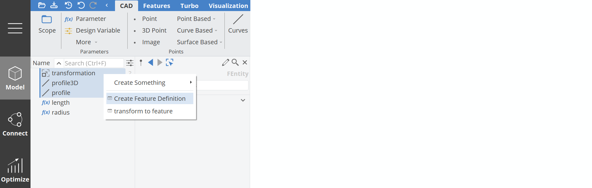
- Select the curves and the transformation (while holding the Ctrl button) and create a Feature Definition via the context menu (right-click) of the selection (do not select the Parameters):
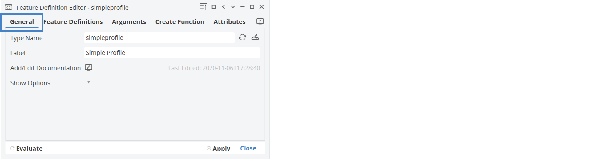
- Set the Type Name to "simpleprofile" (General tab).
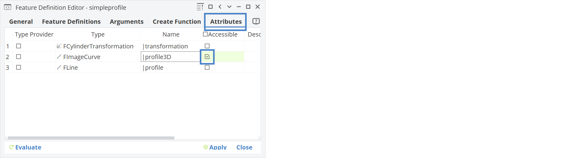
- In the Attributes tab, make only profile3D accessible -- this is our curve of interest for the upcoming Meta Surface.
- Press Apply and close the dialog.
Meta Surface
In this step, a Meta Surface is created. A simple, say, metal sheet results from the basic shape of the profile:
-
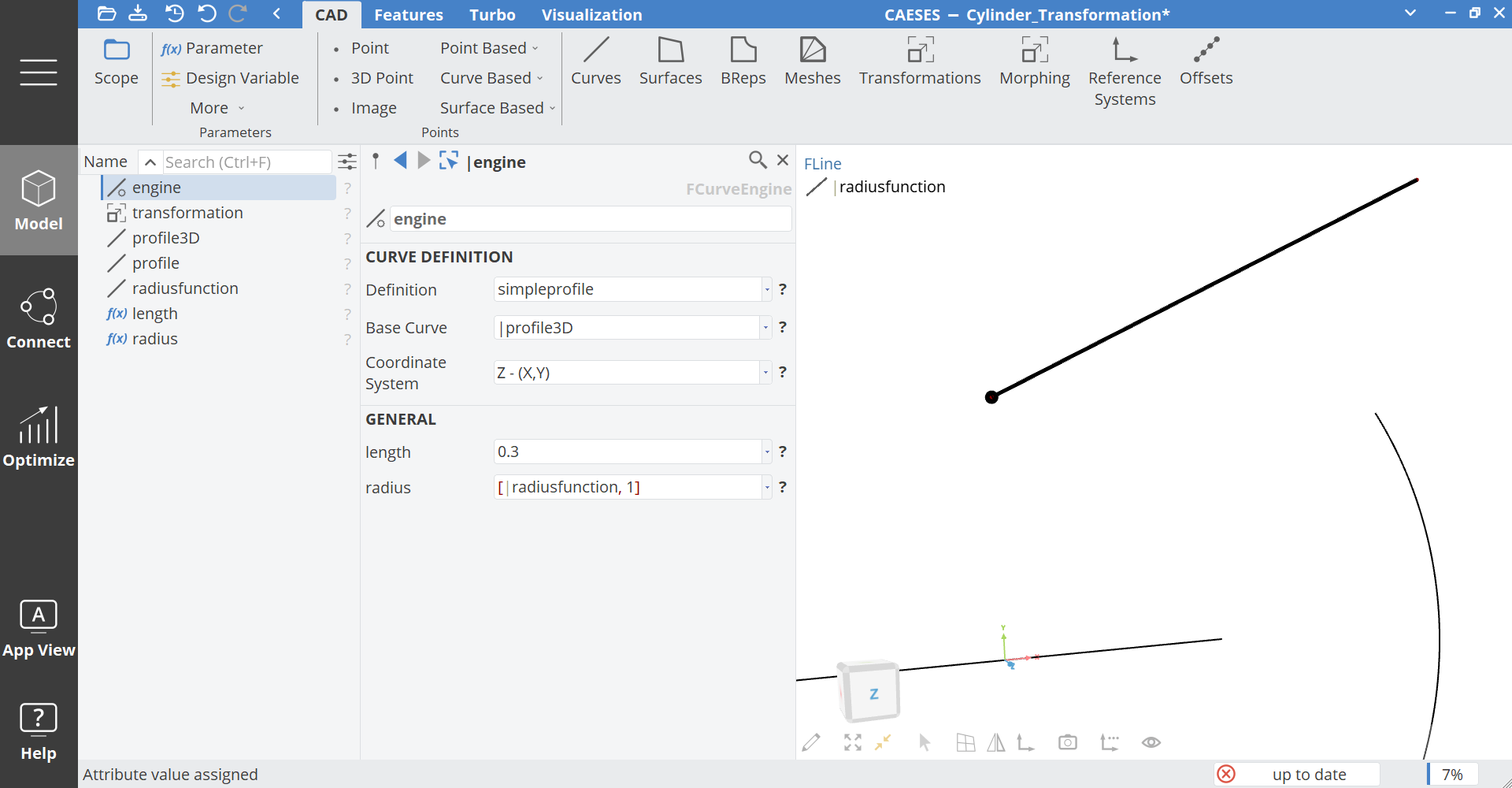
Create a Curve Engine via Model > CAD > Surfaces > Meta Surface > Curve Engine and set its name to "engine".
-
Choose the simpleprofile from the drop-down menu of the Definition attribute
The Base Curve will be set to profile 3D automatically, since we only made this curve accessible.
- Set the attribute length to a constant value of
0.3.
Let's say the hub radius is 0.6 and the tip radius 1. The corresponding radial function can be created and applied as follows:
-
Create a line via Model > CAD > Curves > Line and name it "radiusfunction".
-
Set the Start Position to
[0,0.6,0]. -
Set the End Position to
[1,1,0]. -
Select engine and set this function at the attribute radius. You can either drag and drop the radiusfunction into the field or click into the radius attribute and use the Alt key selection.
-
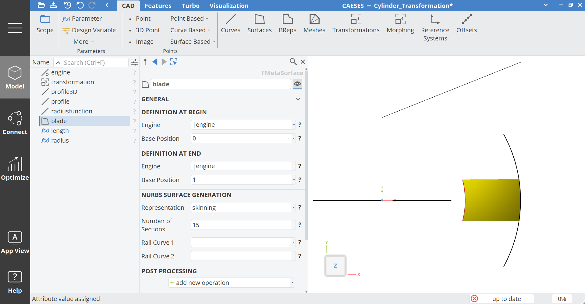
While engine is still selected, create a Meta Surface via Model > CAD > Surfaces > Meta Surface > Meta Surface.
-
Set the name to "blade".
Periodic Visualization
For visualization purposes, we create copies of the blade by using a predefined Feature Definition:
-
Select the surface blade.
-
Go to the Visualization tab (in the Model workspace).
-
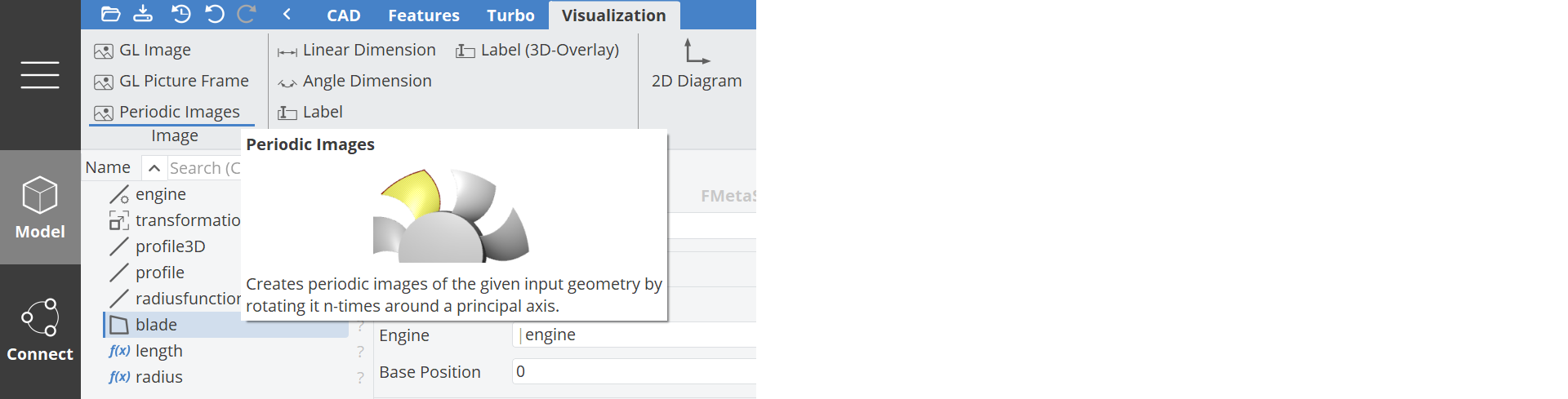
While the blade surface is still selected, create a Periodic Image
-
Set the number of blades (N) to
10. -
Set Axis to Z.
-
Rename the new object periodicimages1 to "fan".
This is only for visualization. The feature does not create new surfaces but only so-called GL-images which cannot be exported. If you need all blades to conduct a CFD analysis then you need to create image surfaces (type FImageSurface).
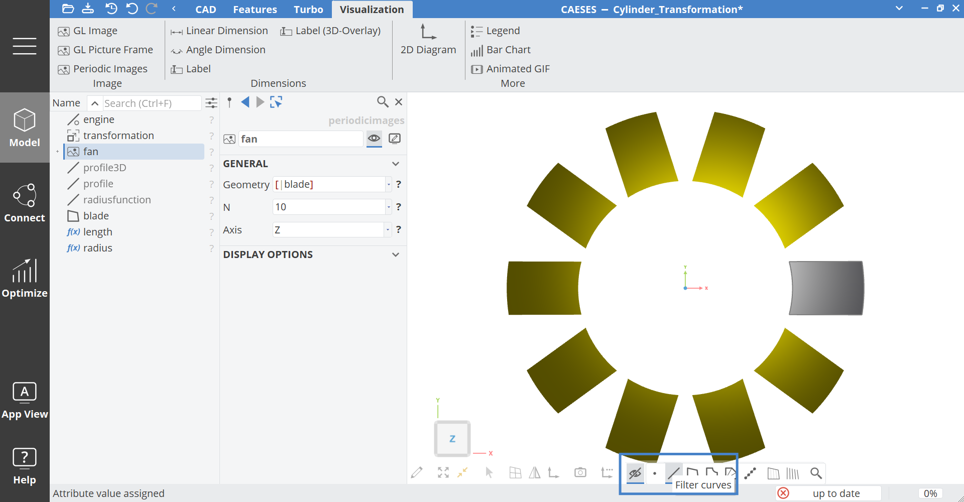
- Activate the Curve Filter at the bottom of the 3D Window to hide the curves
Adding Blade Parameters
So far, our fan is not that exciting since only the profile length can be controlled. In this step, a twist parameter for the blade is introduced. Basically, any new blade parameter needs to be defined in the 2D space (XY-system) of the profile. In order to twist the blade, a rotation needs to be applied to the initial profile.
Let's edit the Feature Definition for our simple profile
-
Go to the Features tab (in the Model workspace)
-
Edit the Feature Definition simpleprofile (e.g. by double-clicking on it).
-
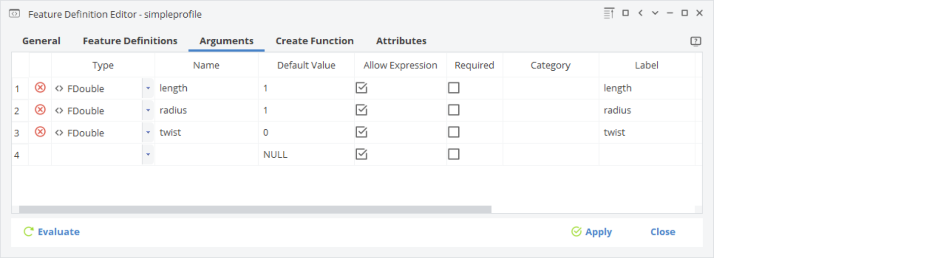
Add another input argument of type FDouble and name it "twist".
-
Set the Default Value to
0.
- In the Create Function tab, add the following lines to your Feature Definition (you can simply copy and paste the code or type it yourself):
rotation dr()
dr.setPrincipalAxis("Z")
dr.setAngle(twist)

imagecurve newprofile()
newprofile.setCurve(profile)
newprofile.setImageTransformation(dr)
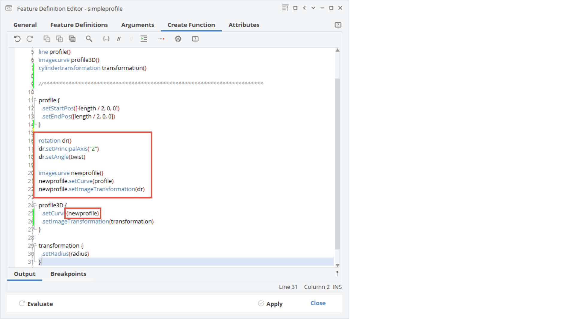
-
Make sure to adapt the input curve for the profile3D. Change it from profile to newprofile
-
Press Apply and close the dialog (optional: check the Accessible tick in the Attribute tab of the Feature Definition again (see one of the previous steps: Feature Definition).
First, a rotation gets defined using twist as angle input. This Rotation is then used in combination with the initial profile to create a new Image Curve. Finally, the new Image Curve (i.e. the rotated profile) is then mapped into the 3D space.
Radial Twist Function
We can now change the value of the twist. Again, this is only a constant value for which we introduce a function in this step.
First, a quick test:
-
Select engine and set a constant value of
45for the new input argument twist. -
If you like, change the number of blades (N) of the Periodic Image fan as well for testing.
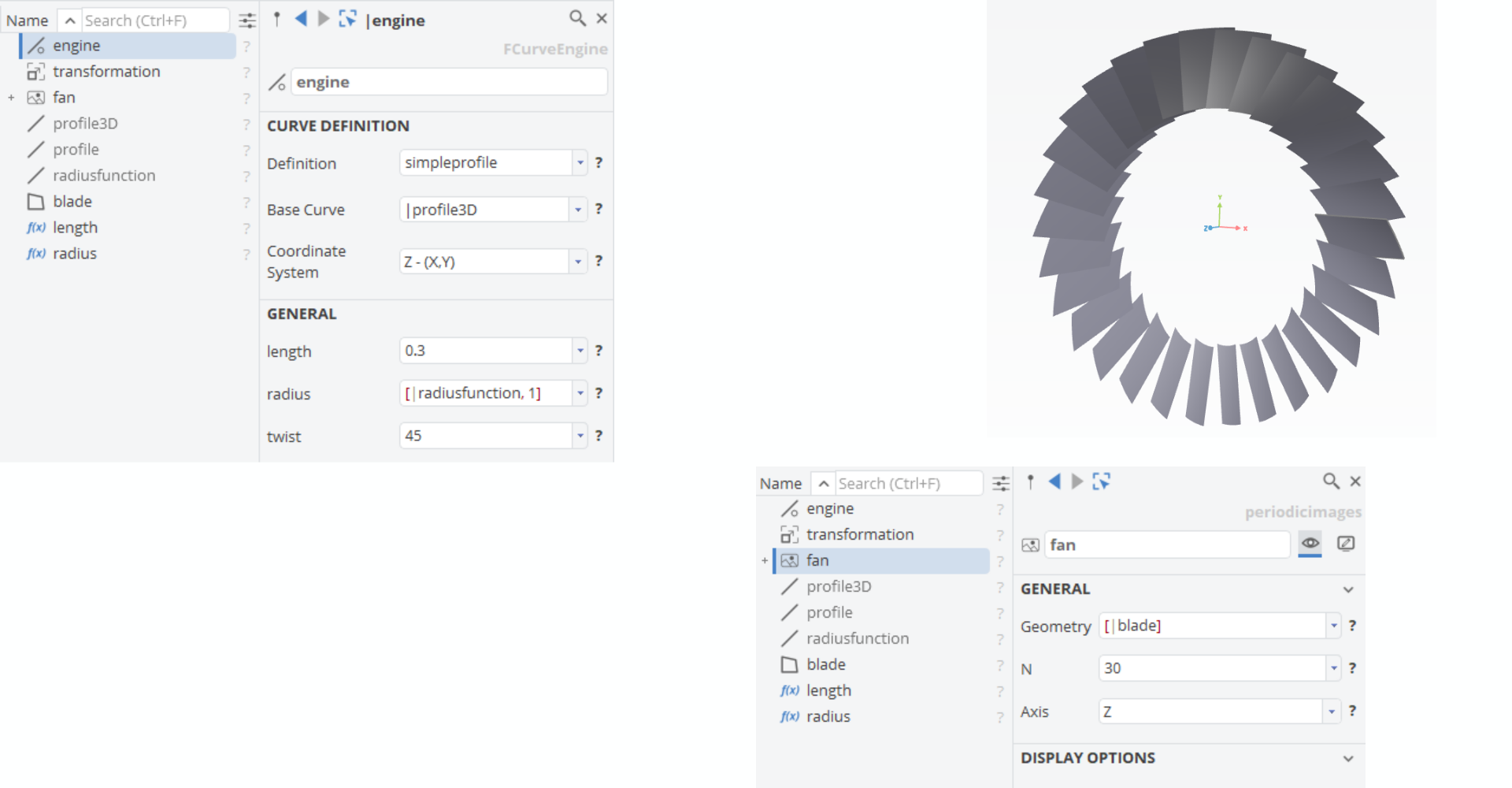
Let's create a function for the twist.
-
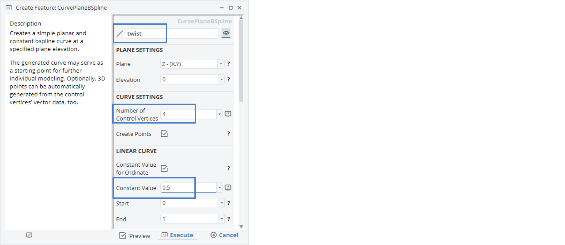
Similar to the previous tutorials, choose e.g. Model > CAD > Curves > Point Based > Planar B-Spline to create an initial Planar B-Spline Curve.
-
Rename CurvePlaneBSpline1 to "twist".
-
Set Number of Control Vertices to
4. -
Set Constant Value to
0.5.
-
Press Execute.
-
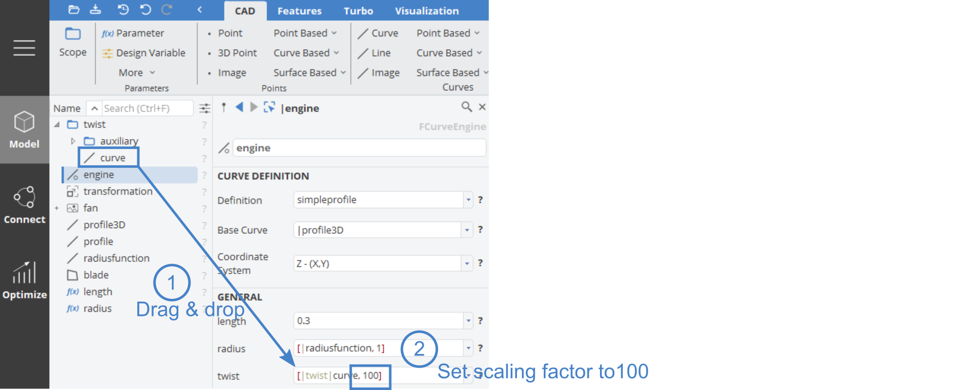
Drag & drop the curve from scope twist into the Curve Engine attribute twist.
-
Set a scaling factor of
100so that the normalized values from the function are multiplied by 100 (e.g. 0.5 * 100 = 50° which is the angle for the twist rotation).
Twisting the Blade
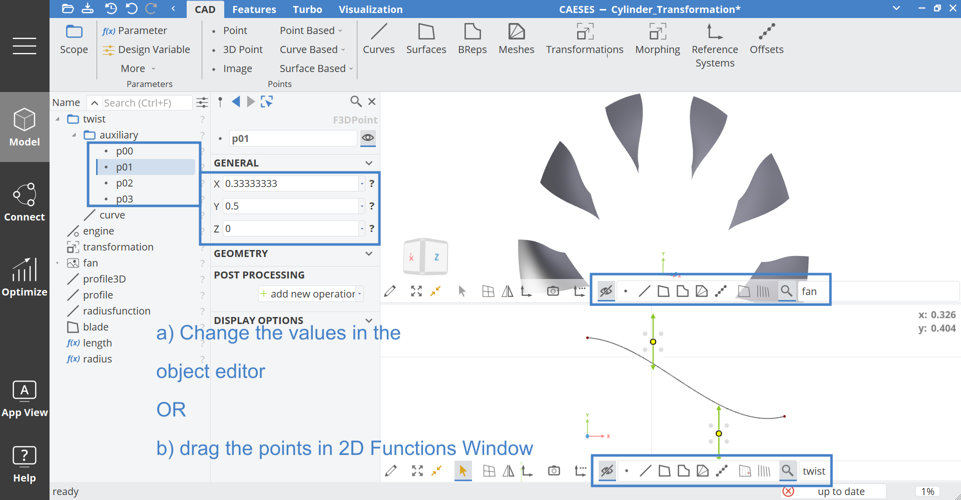
The twist can now be controlled by the twist function. In order to manipulate the twist, we can simply drag and drop the points of the twist function in the 3D View or alternatively change this twist point's coordinates (located in the auxiliary scope) in the object editor.
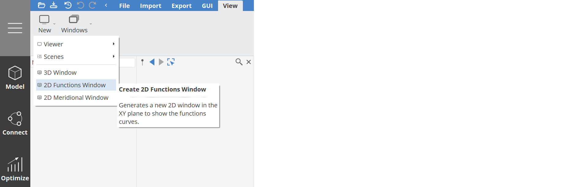
- Let's open a second window within CAESES for our functions via Menu workspace > View tab > New > 2D Functions Window
- Set the name filters of the views for distinct visualization according to the screenshot below
Either:
a) Select one or more points in the scope twist|auxiliary and edit the values in the object editor
or
b) drag the points in the 2D Functions Window
Finalizing
Here are some final remarks for next steps and for finalizing this tutorial on your own:
-
Add a radial function for the profile parameter length and set it at the Curve Engine (see previous step Radial Twist Function). A scaling factor (for twist it was 100) is not required at the Curve Engine. For instance, use copy & paste of the existing twist scope if you like to use the same type of curve (the twist function is a Planar B-Spline). You can also try out different curve types such as the F-Spline Curve for which the tangent angles can be controlled e.g. by Design Variables.
-
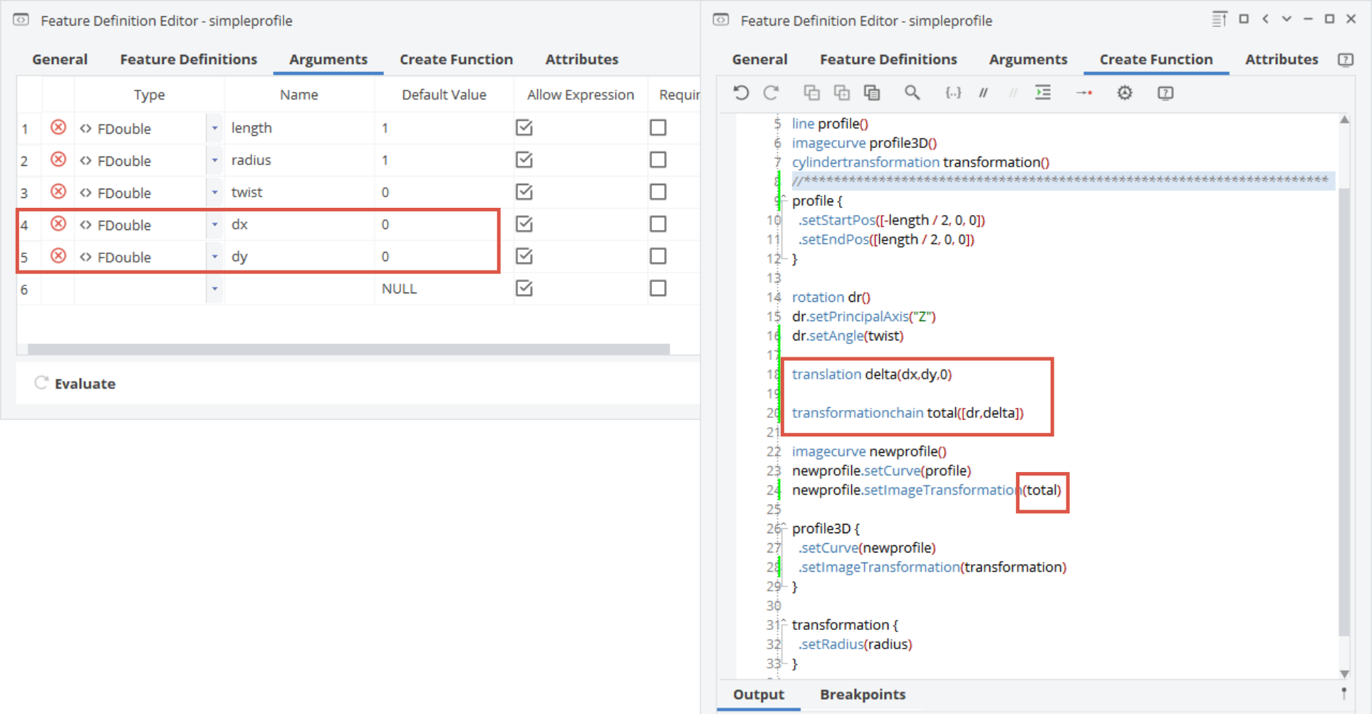
Add two more input arguments for the profile definition to move it in the X- and Y-directions in the 2D plane (say, "dx" and "dy"). Use a Translation object for this purpose. The new Translation (delta with dx and dy) and the Rotation (dr with twist) are then put into a Transformation Chain called "total". This chain is then set as Image Transformation for "newprofile" as shown below:
-
Add radial functions for the new input parameters dx and dy from above and set the curves in the engine.
-
Create a scope called "functions" and put the function curves or scopes twist, dx and dy inside it to organize the object tree.
Although we specified translations in X- and Y-directions (i.e. dx and dy), the actual Cylindrical Transformation implies that dx shifts in tangential direction, and dy shifts in the axial direction. If you like, rename dx and dy accordingly.
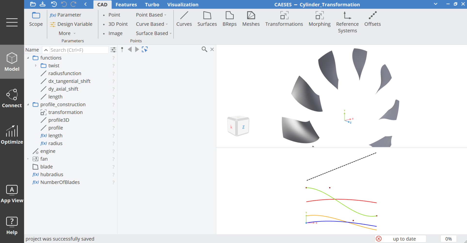
If you want to use another profile definition (and not just a simple line), only the first part of the Feature Definition needs to replaced by a new profile description. If the new profile is also called “profile”, the sequence starting from line 13 in the screenshot will work correctly. Always check the Attributes tab for changes and make sure that your final 3D curve is accessible (profile3D).
CAESES Project File
If you want to take a look at the finalized parametric model you can find the resulting CAESES project file cylinder-transformation.cdb here: