Propeller with Different Profiles
This tutorial explains how to create a propeller in CAESES using the Advanced Propeller Workflow by using different profiles and generating a Profile Surface, which is then used as a Profile Configurator within the Propeller Workflow.
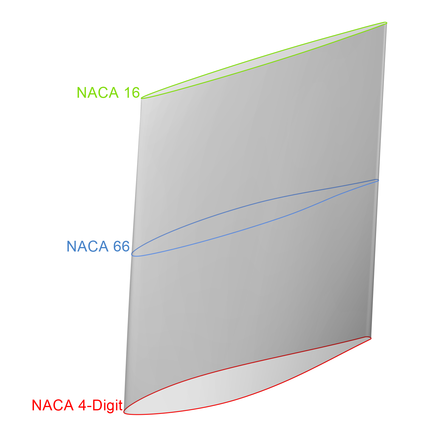
This approach allows you to define multiple profiles along the blade span by creating a Profile Surface that describes the variation of the profile shape from root to tip. For example, you can assign different profiles at the root, mid-span and tip, enabling a more flexible and realistic blade design.
Preparation
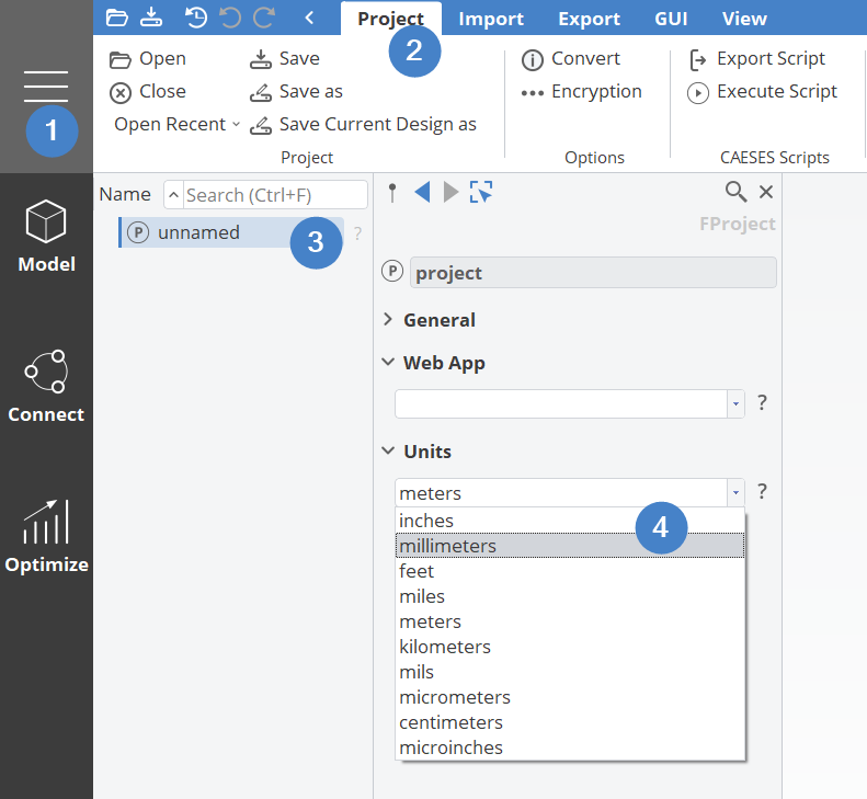
Before starting this tutorial, set the Project Units to millimeters.
To start, navigate to the Model workspace > Propeller tab > Propeller Workflows category > Advanced Propeller Workflow in the Propeller tab of CAESES.

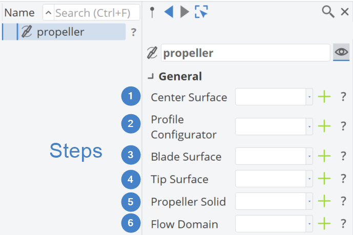
Once clicked, you should see the layout shown below, which provides an overview of the steps required for the Advanced Propeller Workflow.
Center Surface
The first step in the propeller design workflow is defining the Center Surface.
-
Click the plus button next to Center Surface.
- This creates a center surface that incorporates information from various radial distributions, which are typical in propeller design.
-
For each distribution:
- Click the plus button to create a 3rd-degree B-Spline Curve.
- Select the corresponding number of control points.
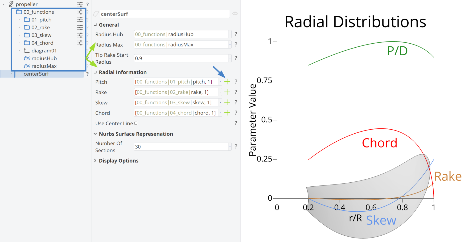
The scope structure for radial distributions follows the naming convention 0x_functionName for Center Surface. Design variables impacting each distribution are organized within their respective scopes.
Radial Distributions
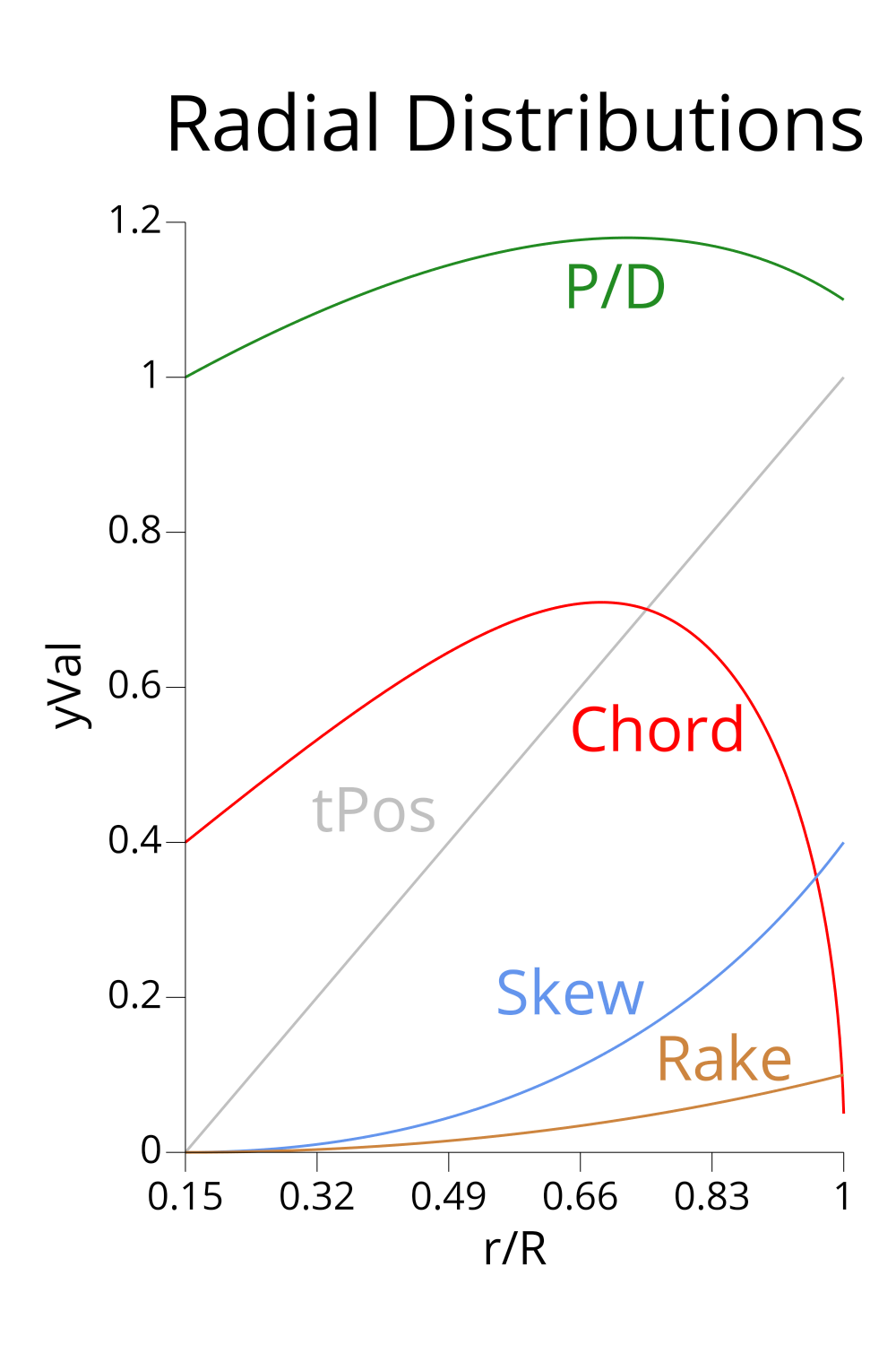
The pitch, rake, skew and chord distributions used in this tutorial are the default ones generated by the Propeller Workflow, configured with the following number of control points. Additionally, the values of some design variables are modified as follows:
-
Pitch Function: 3 control points
pitchRoot = 1.0pitchTip = 1.1
-
Rake Function: 3 control points
rake1 = 0.0
-
Skew Function: 3 control points
skew1 = 0.0skewTip = 0.4
-
Chord Function: 5 control points
chordRoot = 0.4chord1 = 0.6chord2 = 0.9chord3 = 0.4
-
Change the
radiusHubparameter from0.2to0.15.
Profile Configurator - Surface Component
By selecting the Propeller Component in the Object Tree and clicking the plus button next to the Profile Configurator, three options will appear:
- Profile Configurator via Camberline and Thickness
- Profile Configurator based on Profile Import
- Profile Surface with different Profiles
Select the Profile Surface with different Profiles option.
Once selected, the corresponding GUI will appear in the Object Editor.
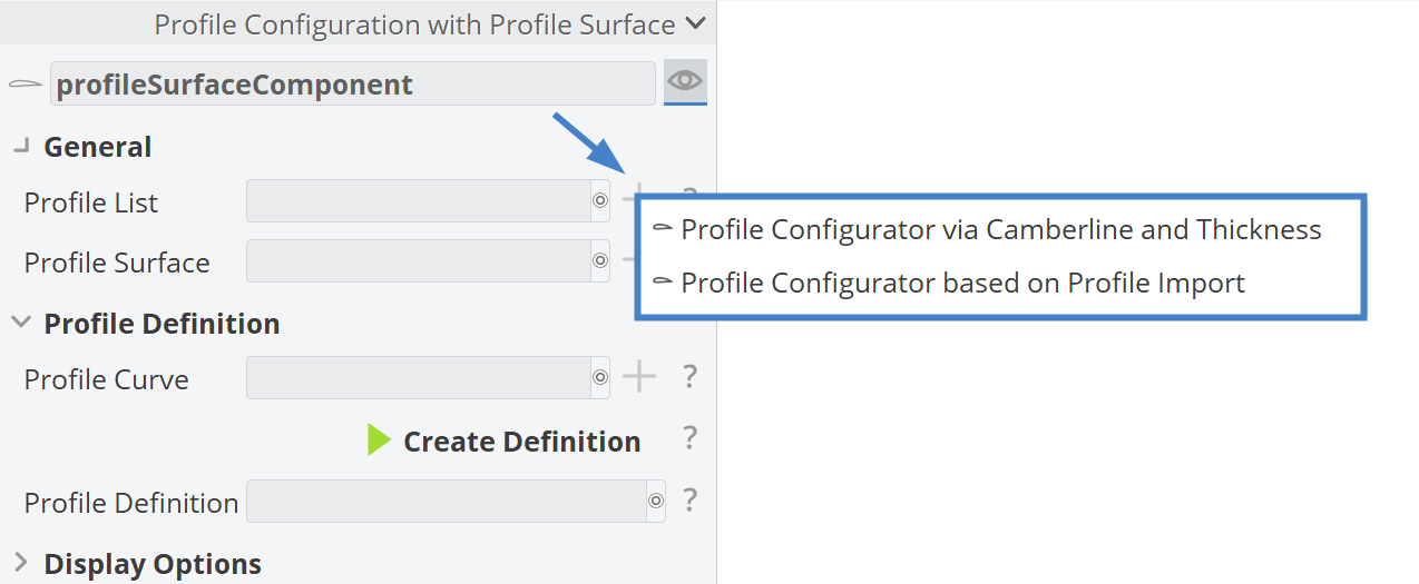
First, click the greem plus (+) button next to Profile List. A new window will appear with two options:
- Profile Configurator via Camberline and Thickness
- Profile Configurator based on Profile Import
The goal here is to create multiple Profile Configurators. In this tutorial, we will use profiles defined via Camberline and Thickness Distribution. However, you can also use Profile Configurators based on Import if preferred (see: Import Propeller Profiles Tutorial).
You can create as many Profile Configurators as needed, but it is recommended to keep the number low for clarity and manageability. In this tutorial, we will use three. Each time you want to create a new one, click the plus (+) button next to Profile List.
Profile List
Once the previously mentioned plus (+) button is clicked under the profileSurfaceComponent, two new Objects are generated: one named profileConfigurator_1 and the other is a Parameter named position_1 with a value of 0.
In the Profile List, a new element is now added that contains two sub-elements: the Profile Configurator and its corresponding position.
The position of each Profile Configurator ranges from 0 to 1, representing its spanwise location along the blade. The following profiles will be used in this tutorial:
0corresponds to the root of the blade - NACA 4-Digit0.5to the mid-span - NACA 661to the blade tip - NACA 16
The position of the Profile Configurator indicates the spanwise location on the blade, where the cylindrical section exactly matches the properties of the corresponding Profile Configurator. The regions between different profiles are smoothly interpolated based on the preceding and following profiles.
Profile 1 (Root): NACA 4-Digit
A NACA 4-Digit profile is used at the root of the blade because they are well tested thick, strong and the region lift demand is low and cavitation risk is minimal.
In order to generate such a profile, follow these steps:
- Click the plus (+) button next to Profile List in profileSurfaceComponent
- Click the plus (+) button next to Camberline in profileConfigurator_1
- Select Camberline of NACA 4 Digits from the pop-up window
- Click the plus (+) button next to Thickness Curve in profileConfigurator_1
- Select Thickness Distribution of NACA 4 Digit Modified from the pop-up window
- Click the plus (+) button next to Profile Curve in profileConfigurator_1
Now everything is set up for the Profile Configurator and under profileConfigurator_1, three scopes are available:
- 01_camber
- 02_thickness
- 03_profile
Profile 2 (Mid-span): NACA 66
A NACA 66 profile is used at the mid-span of the blade because it offers a good balance of high lift, low drag and cavitation resistance, making it ideal for the region where most of the thrust is generated.
To generate such a profile, follow these steps:
- Click the plus (+) button next to Profile List in profileSurfaceComponent
- Change the value of position_2 under profileSurfaceComponent from
0to0.5 - Click the v next to Camberline in profileConfigurator_2
- Select Camberline NACA a=08 modified from the pop-up window
- Click the plus (+) button next to Thickness Curve in profileConfigurator_2
- Select Thickness Distribution for NACA 66 from the pop-up window
- Click the plus (+) button next to Profile Curve in profileConfigurator_2
Under profileConfigurator_2, three scopes for the camber, thickness and profile are available.
Profile 3 (Tip): NACA 16
A NACA 16 profile can be used near the tip of the blade due to their moderate thickness and good laminar flow characteristics.
To generate such a profile, follow these steps:
- Click the plus (+) button next to Profile List in profileSurfaceComponent
- Change the value of position_3 under profileSurfaceComponent from
0to1 - Click the plus (+) button next to Camberline in profileConfigurator_3
- Select Camberline of NACA 16 from the pop-up window
- Click the plus (+) button next to Thickness Curve in profileConfigurator_3
- Select Thickness Distribution for NACA 16 from the pop-up window
- Click the plus (+) button next to Profile Curve in profileConfigurator_3
Under profileConfigurator_3, three scopes for the camber, thickness and profile are available.
Profile Surface
Once the Profile List is complete, you need to generate a Profile Surface from this list. The Profile Surface extends in the span-wise direction from 0 to 1 (based on the position parameters) and in the chord-wise direction, it also ranges from 0 to 1. This results in a normalized profile surface without a direct relation to the actual chord length.
The Profile Surface is essentially a Lofted Surface with smooth blending, created by interpolating the profile curves at the defined positions, as shown in the figure below.
To create the Profile Surface, go to the profileSurfaceComponent GUI and click the plus (+) button next to Profile Surface, as shown below.
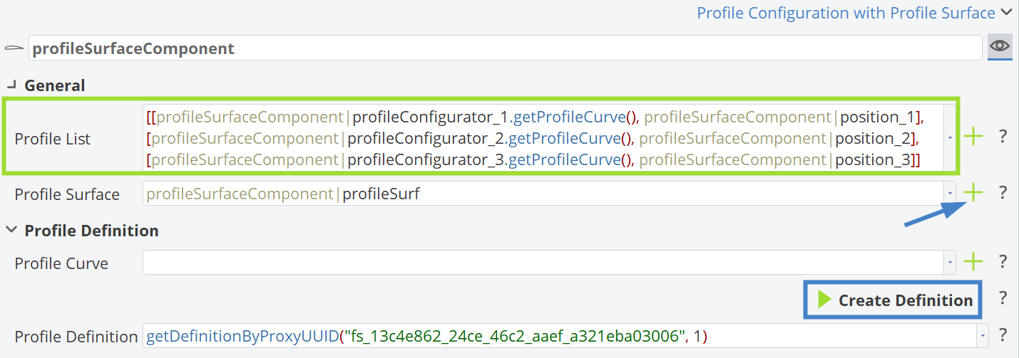
The Profile Surface is then generated based on the Profile List (shown in the image above). From this surface, you can generate the corresponding Profile Definition by clicking the Create Definition button. A seemingly random name will appear in the GUI; this is internal to CAESES and fully functional, even though it might look unusual.
When using a Profile Surface, a Profile Curve is not required in the Propeller Workflow.
Blade Surface
In the Propeller Component GUI, continue by clicking the plus (+) button for the Blade Surface, then select Blade Surface again.
This action creates the following three objects:
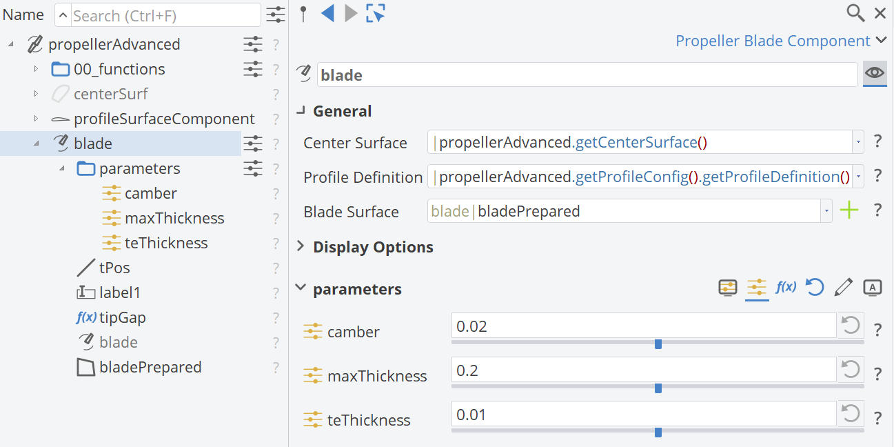
blade(type:FPropellerBlade)tipGap(type:FParameter)bladePrepared(type:FImageSurface)
To continue the process that follows, you will need to make the blade (type: FPropellerBlade) invisible by clicking on the icon in the object tree to hide the blade in the 3D view.
Parametric Position Curve
In order for the info from the Profile Surface to be properly transferred to the propeller blade, a Linear Distribution is needed. This transfers the info from the parametric space [0,1] to the normalized geometric space [radiusHub, radiusMax]. It functions as a curve that maps this. For that reason, you need to create a Line Curve under the blade component named tPos with the following properties:
- Starting Point:
[|propellerAdvanced|00_functions|radiusHub, 0, 0] - Ending Point:
[|propellerAdvanced|00_functions|radiusMax, 0, 0]
Now, all the radial distributions used in this tutorial are shown together in the figure below.
Parameters
At this step, you will need to parametrize the Profile Surface in a rational and smooth and meaningful way without many design variables.
For that purpose you need to the following:
- Create Scope named parameters under the blade Component
- Create Design Variable named camber
- Default Value:
0.02 - Lower Bound:
0 - Upper Bound:
0.04
- Default Value:
- Create Design Variable named maxThickness
- Default Value:
0.2 - Lower Bound:
0.15 - Upper Bound:
0.25
- Default Value:
- Create Design Variable named teThickness
- Default Value:
0.01 - Lower Bound:
0.0075 - Upper Bound:
0.0125
- Default Value:
- Create Design Variable named camber
Having a complex methodology like this, the number of design variables is kept small without compromising the variety of resulting shapes. Below is shown how to connect the above Parameters with the Profile Configurators from the previous Section, where you can clearly observe the pattern. In this way, we indirectly create distributions for the Profile Parameters.
Camber Parametrization
For parametrizing the camber of the Profile Surface, you need to do the following:
- Go to profileConfigurator_1 under profileSurfaceComponent
- Go to the 01_camber scope under profileConfigurator_1
- Change the value of camber to
-|propellerAdvanced|blade|parameters|camber / 2
- Go to profileConfigurator_2 under profileSurfaceComponent
- Go to the 01_camber scope under profileConfigurator_2
- Change the value of camber to
|propellerAdvanced|blade|parameters|camber
- Go to profileConfigurator_3 under profileSurfaceComponent
- Go to the 01_camber scope under profileConfigurator_3
- Change the value of camber to
0
Thickness Parametrization
For parametrizing the maximum and trailing edge thickness of the Profile Surface, you need to do the following:
- Go to profileConfigurator_1 under profileSurfaceComponent
- Go to the 02_thickness scope under profileConfigurator_1
- Change the value of maxThickness to
|propellerAdvanced|blade|parameters|maxThickness - Change the value of teThickness to
|propellerAdvanced|blade|parameters|teThickness
- Go to profileConfigurator_2 under profileSurfaceComponent
- Go to the 02_thickness scope under profileConfigurator_2
- Change the value of maxThickness to
2 * |propellerAdvanced|blade|parameters|maxThickness / 3 - Change the value of TEThickness to
2 * |propellerAdvanced|blade|parameters|teThickness / 3
- Go to profileConfigurator_3 under profileSurfaceComponent
- Go to the 02_thickness scope under profileConfigurator_3
- Change the value of maxThickness to
|propellerAdvanced|blade|parameters|maxThickness / 4 - Change the value of TEThickness to
|propellerAdvanced|blade|parameters|teThickness / 2
FPropellerBlade
By selecting the blade object (type FPropellerBlade), you can see the GUI in the Object Editor, here you need to parse the input for the Profile Parameters for the Profile Surface and Pos, as figured below.
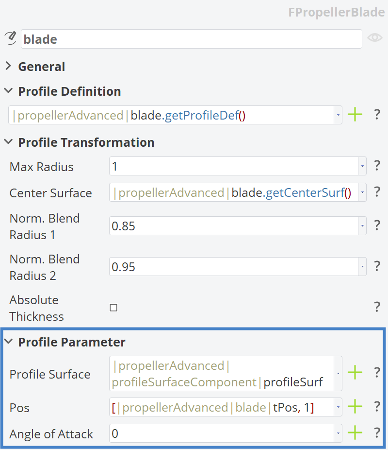
Now you can make the blade (type: FPropellerBlade) visible again by clicking on the greyed-out icon in the object tree.
Blade Scope Structure
Everything in place, the figure below illustrates the scope structure along with the blade Component GUI inside CAESES.
Tip Surface
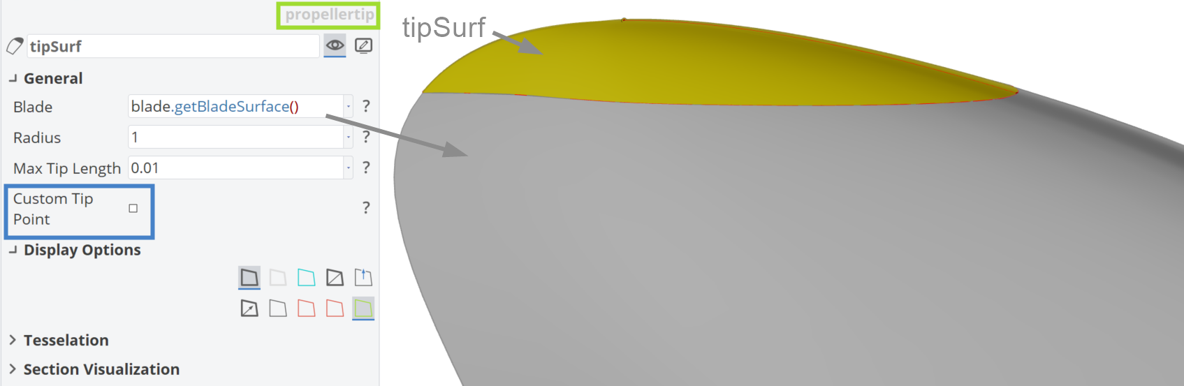
Here, the Tip Surface is created by clicking the plus button in the propeller component GUI. The following properties are automatically configured for this setup:
- Source:
|propeller.getBladeSurface().getBladeSurface() - Radius:
1 - Max Tip Length:
0.01
Below is a figure showing the tip region of the blade. The main part of the blade is depicted in gray , while the tip surface is highlighted in yellow color.
Propeller Solid
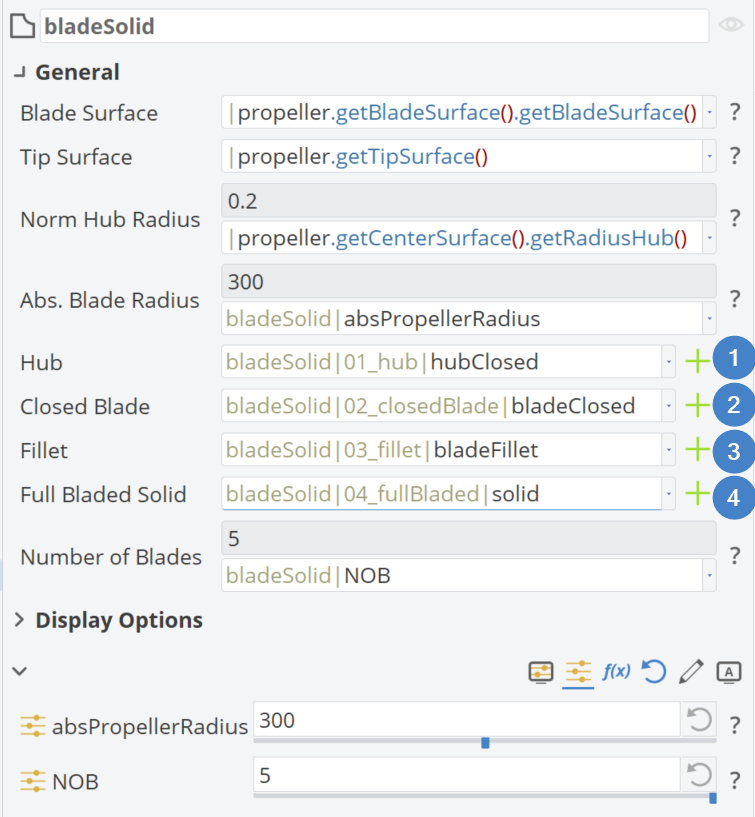
Following the creation of the blade and tip surfaces, the next step is to create a watertight, closed solid geometry.
- Click the plus button in the propeller component.
- This will generate a bladeSolid component along with two design variables named absPropellerRadius and NOB.
- These correspond to the propeller radius and the number of blades (NOB).
- Set the range of absPropellerRadius from
100to5000millimeters, with a default value of2500. - Keep the range of NOB from
3to5, with a default value of4.- Set it as an integer design variable.
- Next, create a parameter under the bladeSolid component named "D".
- This corresponds to the Diameter with the expression:
D = absPropellerRadius * 2.
- This corresponds to the Diameter with the expression:
Steps for Propeller Solid Creation
The steps to complete these tasks are illustrated in the figure below.
Hub
By clicking the corresponding plus button in the bladeSolid GUI, you can create a hub BRep scaled to the propeller's radius. For this tutorial, the auto-configured hub from the workflow is sufficient.
Closed Blade
Afterward, you can create a Closed Blade as a BRep in a similar manner. This is achieved through an Operation: boolean|solid from intersections of a scaled version of the blade & tip surface to the propeller radius, combined with a scaled-down version (99%) of the hub geometry, named hubSmall.
Variable Radius Fillet
Having BReps for the blade and the hub correspondingly, then we can move on to the Variable Fillet creation. A rule of thumb that we use for the fillet is to introduce fillet radius on the pressure side 2/3 times compared to max. profile thickness at the root and 1/3 times on the suction side accordingly. Also, the fillet should follow the thickness at the TE and the LE. Based on the aforementioned the following Parameters are defined:
- filletScalefactor =
10 - radiusLe =
thicknessRoot / 10 - radiusSide1 =
thicknessRoot / 3 - radiusSide2 =
thicknessRoot * 2 / 3 - radiusTe =
thicknessTE / 2 - thicknessRoot =
|propellerAdvanced|00_functions|04_chord|chordRoot * |propellerAdvanced|blade|functions|maxThickness_distribution|maxThickness_00 * |propellerAdvanced|bladeSolid|D - thicknessΤe =
|propellerAdvanced|00_functions|04_chord|chordRoot * |propellerAdvanced|blade|functions|teThickness * |propellerAdvanced|bladeSolid|D
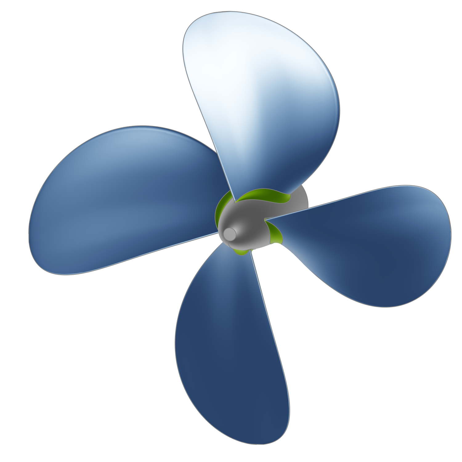
Full Bladed
The final step in the Propeller Solid process is to generate the complete propeller geometry, with all blades smoothly connected to the hub as a single BRep, as shown in the figure below.
Conclusion
This tutorial demonstrates how to use different profiles for blade generation within the Advanced Propeller Workflow in CAESES.
From these profiles, a Profile Surface is generated, which is parametrized with and reflects their geometric influence on the propeller blade.
The Profile Surface parametrization uses a few design variables but provides a great variety of shapes, showcasing and highlighting the power of this design methodology.
This approach enables users to generalize the propeller design workflow in CAESES, making it more flexible and capable of handling more complex geometries that better represent real-world propellers.
CAESES Project File
If you want to take a look at the finalized parametric propeller model to gain a clearer understanding of the concepts presented, you can find the resulting CAESES project file propeller-different-profiles.cdb here: