Import Propeller Profiles

PropellerThis functionality requires the Propeller add-on to be enabled. 5.3.0This functionality requires CAESES version 5.3.0 or later.

This tutorial explains how to create a propeller in CAESES using the Propeller Workflow by importing a 2D profile from an ASCII file (e.g., .dat format) or by importing an existing profile as a Curve, and using it as a Profile Configurator within the Propeller Workflow.

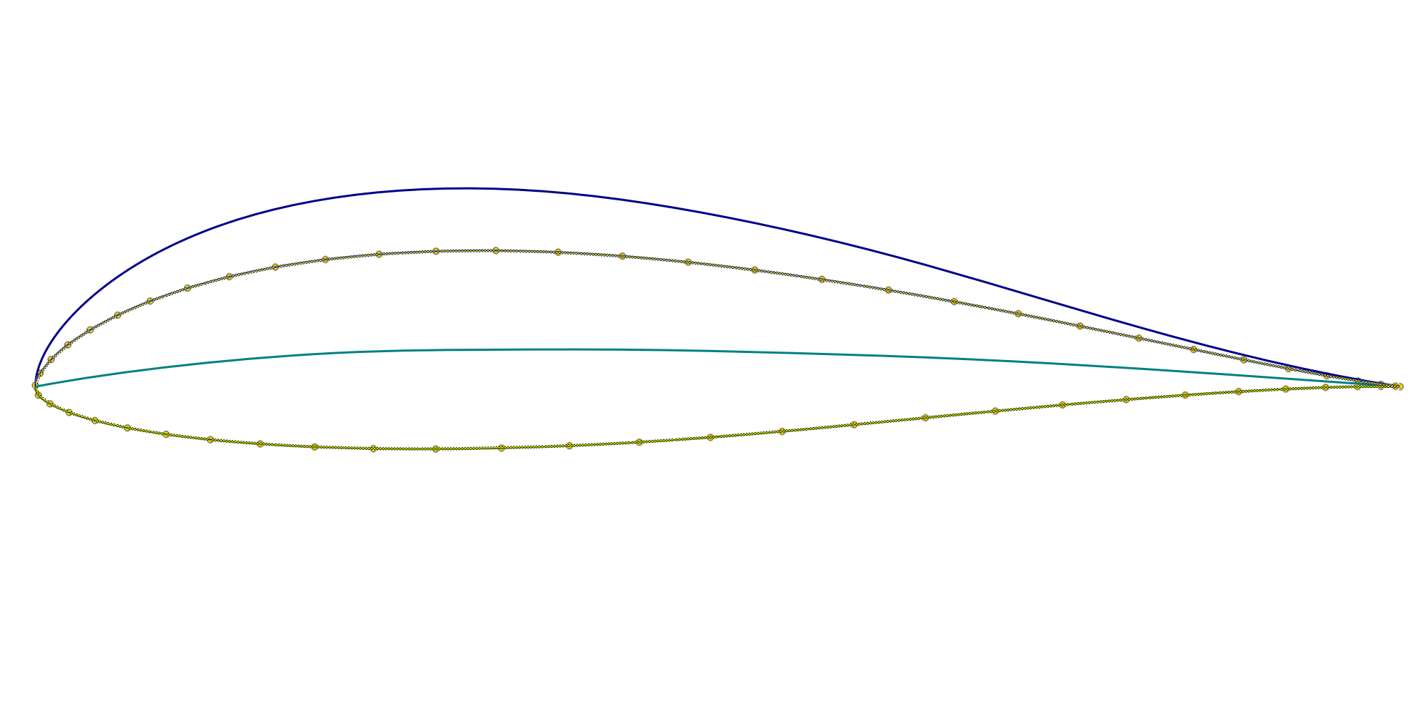
This allows you to retrieve all geometric information from the file and properly parametrize the profile geometry — including camber, thickness distribution and trailing edge (TE) details.

A large collection of airfoil profiles is available from the UIUC Applied Aerodynamics Group.

Preparation

For this tutorial, we use the S2027 low Reynolds number airfoil, which can be downloaded directly:

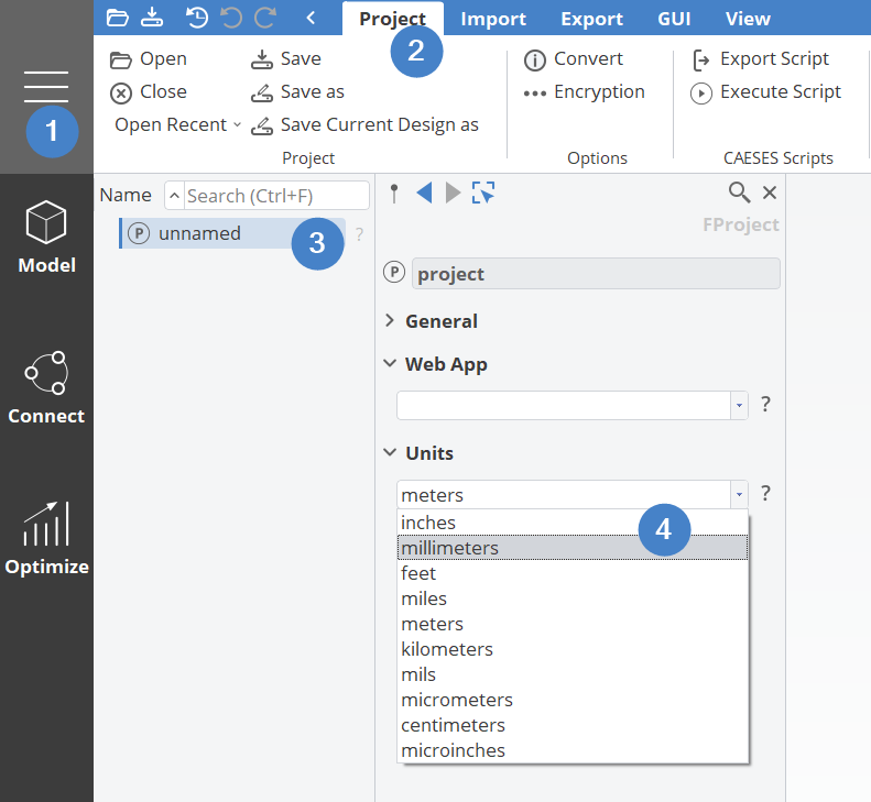
Download S2027 Profile Point Data

set project units

Before starting this tutorial, set the Project Units to millimeters.

To start, navigate to the Model workspace > Propeller tab > Propeller Workflows category > Advanced Propeller Workflow in the Propeller tab of CAESES.

Once clicked, you should see the layout shown below, which provides an overview of the steps required for the Advanced Propeller Workflow.

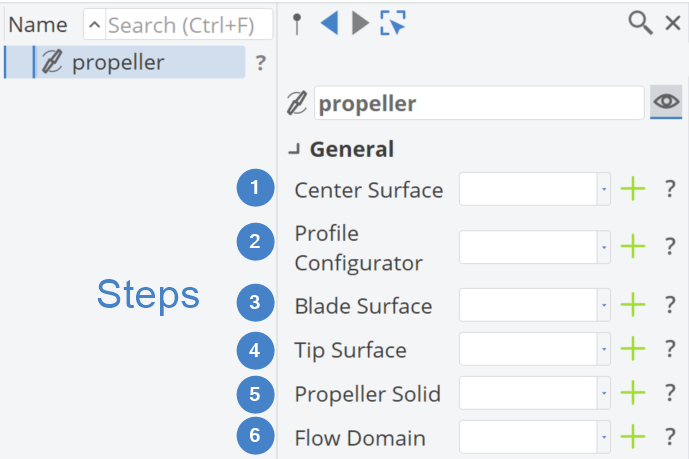
Center Surface

The first step in the propeller design workflow is defining the Center Surface.

• Click the plus button next to Center Surface.
  • This creates a center surface that incorporates information from various radial distributions, which are typical in propeller design.
• For each distribution:
  • Click the plus button to create a 3rd-degree B-Spline Curve.
  • Select the corresponding number of control points.

info

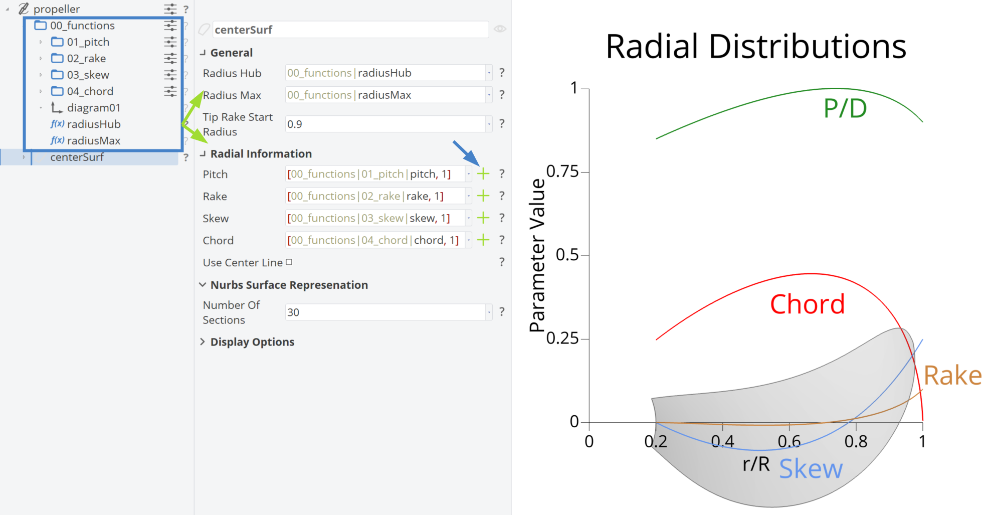
The scope structure for radial distributions follows the naming convention 0x_functionName for Center Surface. Design variables impacting each distribution are organized within their respective scopes.

Radial Distributions

The pitch, rake and skew distributions used in this tutorial are the default ones generated by the Propeller Workflow, configured with the following number of control points:

• Pitch Function: 3 control points
• Rake Function: 4 control points
• Skew Function: 3 control points
• Chord Function: 5 control points

The chord distribution is created using 5 control points. However, the values of the design variables corresponding to the Y-values of some control points have been customized as follows. Set the

• chordRoot-Y to 0.40,
• chord1-Y to 0.52,
• chord2-Y to 0.80.

Profile Configurator

By selecting the Propeller Component in the Object Tree and clicking the plus button next to the Profile Configurator, three options will appear:

• Profile Configurator via Camberline and Thickness

• Profile Configurator based on Profile Import

• Profile Surface with Profiles

• Select the Profile Configurator based on Profile Import option. Once selected, the corresponding GUI element will appear in the Object Editor.

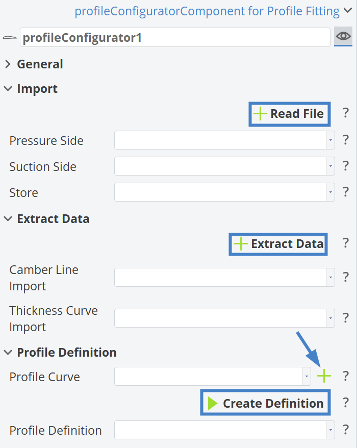
Read File

Click the Read File button and a Scope, named 01_ReadProfile will be created under the Profile Configurator.

Read Profile

In the figure below, the scope structure of 01_ReadProfile is shown on the left and on the right, the input arguments used to read the profile from an ASCII file is displayed.

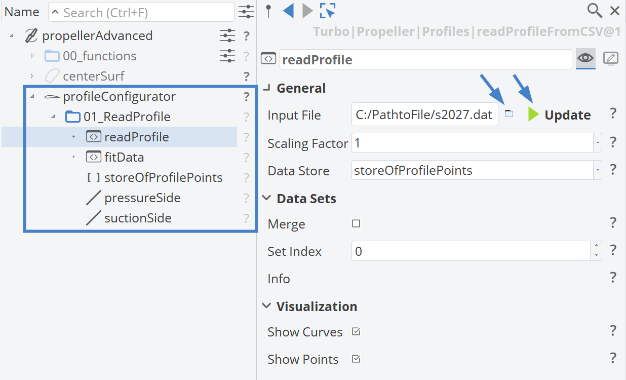
• Click the Scope icon (next to the Input File field that is marked with a blue arrow) to select the profile file from your system.
• Click the Update button next to the Input Field after setting the file.

Once the file is loaded into the CAESES project, the Data is stored in the storeOfProfilePoints FDataStore object.
At this point, the profile information is embedded in the project and the external file is no longer required.

info

Regarding the Data Sets section: If the file contains individual blocks of data (e.g., suction side, pressure side, camber and thickness), the data will be split automatically.

Fit Data

In this step we use the fitData functionality, which separates the pressure and suction sides of the profile into two different curves.

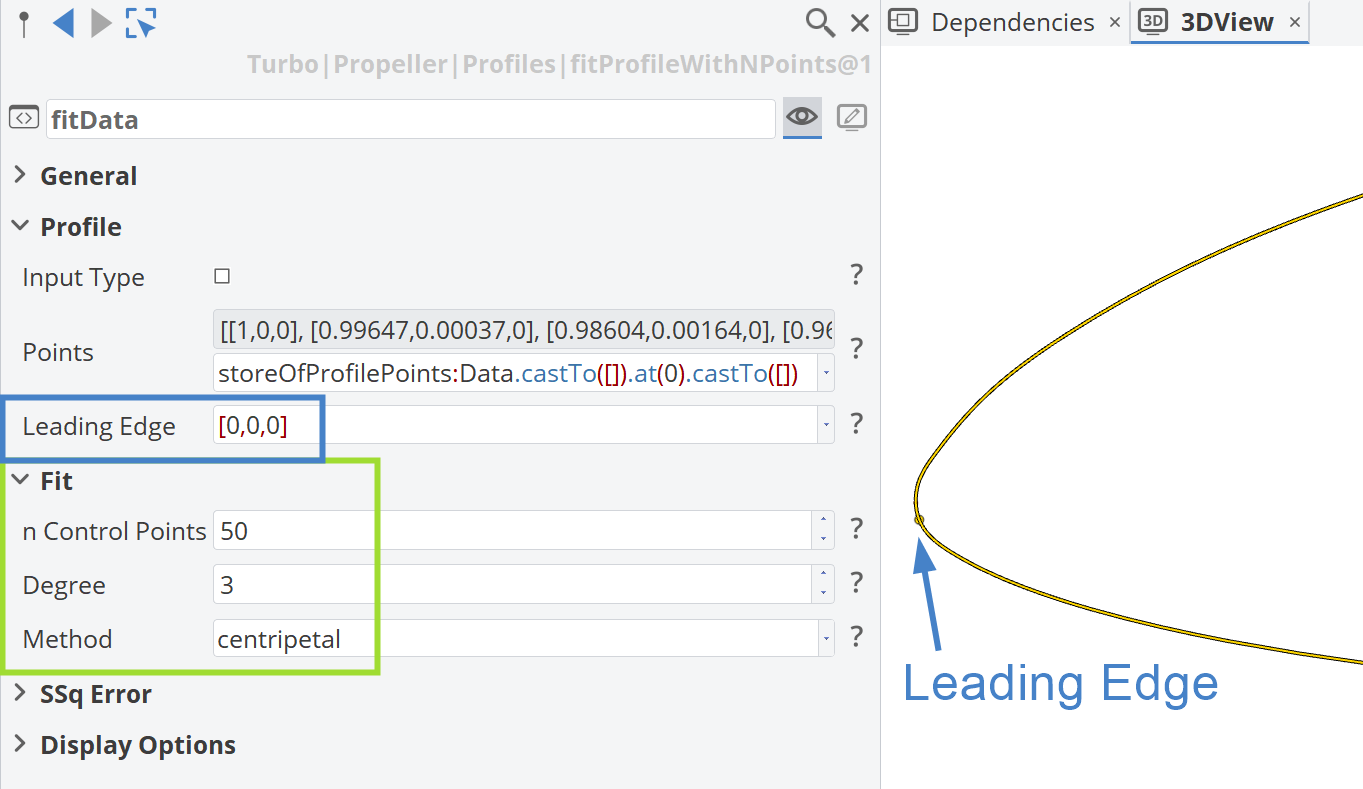
As shown, in the figure below the points are automatically stored. Then the user needs to set the leading edge position, which is usually located at [0,0,0].

Also, by expanding the Fit category, you will find three options that control how the pressure and suction side curves of the profile are fitted using Interpolation Spline Curves:

• Number of Control Points: This is set to 50 by default. If you notice oscillatory behavior in the fitted curve, it may be due to overfitting — in that case, try reducing the number of control points. Conversely, if the spline is too coarse or fails to capture key features, you can increase the number (however 50 control points is already a relatively high number for most cases).

• Degree: This refers to the degree of the spline curve. A value of 3 (cubic spline) is typically used, as it provides a good balance between smoothness and flexibility. You can experiment with other degrees to see which setting best fits your profile geometry.

• Interpolation Method: Two methods are available: chord length and centripetal. The centripetal method is generally more robust and tends to produce better results, especially when fitting complex or unevenly spaced profile points.

tip

If no curve appears, try adjusting the number of control points because the current input may not be sufficient to generate a valid curve.

Curve as Input Type

There is an option to import a curve directly into this workflow instead of using an ASCII file. This can be done by checking the checkbox Input Type, which will show additional input fields as displayed in the figure below.

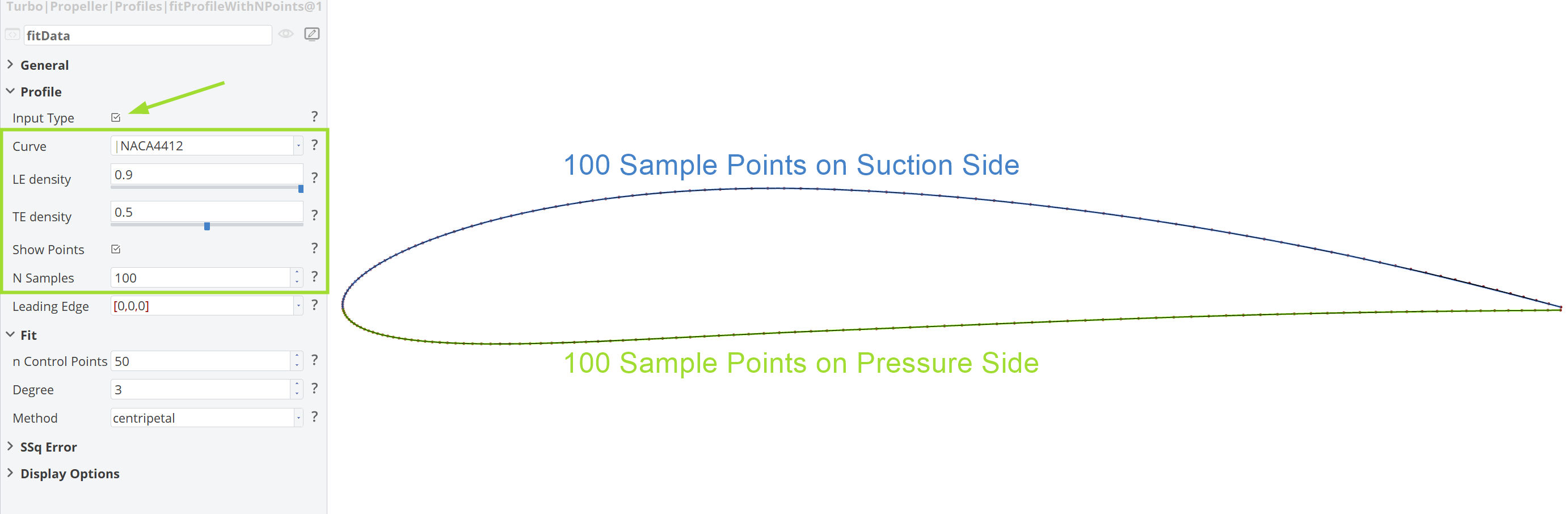
Here, you need to provide a curve as input. In this example, it is a NACA4412, which can be imported geometry or something you designed in CAESES. Then you set the N Samples, which is the number of points on the pressure side and suction side respectively. You can control the distribution of points along the curve using the sliders. Normally, due to the geometry of the profile, you will need more points closer to the Leading Edge and fewer points near the Trailing Edge.

note

If the Input Type field is checked, the readProfile feature becomes redundant since no file needs to be read to retrieve the profile data.

Extract Camber and Thickness

In this step we will extract the camber and thickness data from the imported profile data.

• Go to the Profile Configurator and, in the Object Editor, click the Extract Data button.

This will automatically generate a new Scope named 02_extractCamberAndThickness, which contains the extractCamberAndThickness feature. This feature takes the suction and pressure side curves of the profile as input and extracts the Camber Curve and Thickness Distribution.

Within the same scope, two curves are created: cleanCamber and cleanThickness. You can modify the number of control points and the spline degree, just as described earlier. Additionally, you can define how many sampling points are used when extracting data from the suction & pressure side curves (i.e., the number of points used to sample the source geometry).

This setup is shown in the figure below, which includes typical default values generated by the workflow:

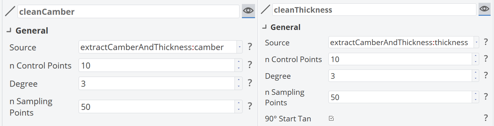
For the Thickness Distribution, you can enable an option to apply a 90-degree tangency at the start of the curve, which is a common requirement for accurate representation of the leading edge region in profile geometries.

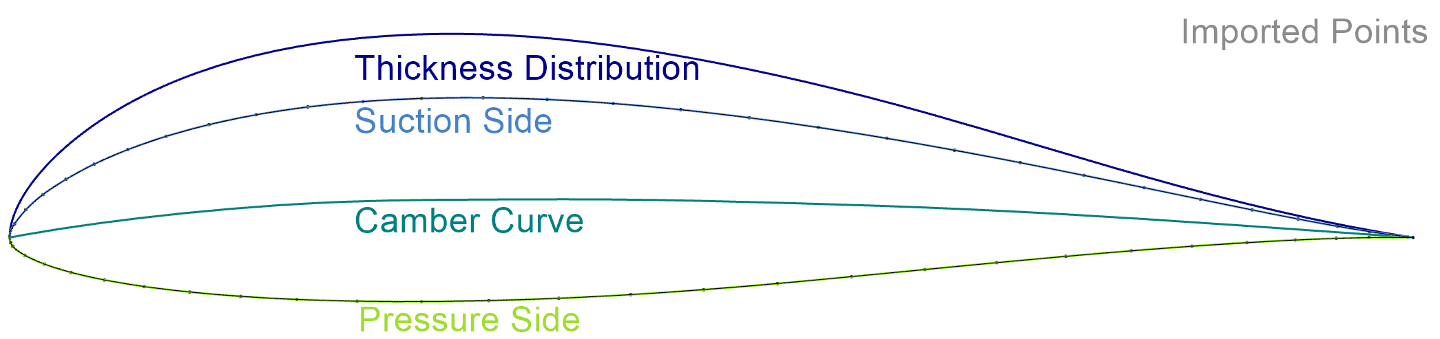
In the figure below, you can see how the pressure and suction side curves properly interpolate the imported Points data and how the Thickness Distribution and the Camber Curve are derived from these two profile curves.

Profile Definition

The next step in completing the imported propeller profile setup is to return to the Profile Configurator and click the plus (+) button next to the Profile Curve. This will create a new profile curve based on the previously extracted Camber and Thickness data.

A new Scope named 03_profile is automatically generated. This scope includes the section curve and a set of parameters that control its shape:

• camber: Maximum camber of the profile
• camberPos: Position of the maximum camber along the x-axis
• maxThickness: Maximum thickness of the profile
• maxThicknessPos: Position of the maximum thickness along the x-axis

Under this scope, you need to create a parameter named "teThickness" with a value of 0.01.

• teThickness: Trailing edge thickness of the profile

Then you can connect this parameter to the section curve. In the Object Editor shown below, under Trailing Edge Shape category, enable Enforce Minimum Thickness and assign the teThickness parameter to the Minimum Thickness Value (marked in blue rectangle). The other parameters are auto-connected (marked in green rectangle).

note

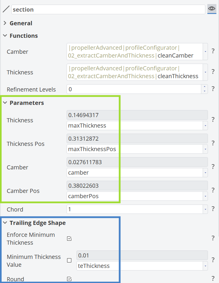
You can also increase the Refinement Levels under the Functions category to add additional knots to the resulting section curve.

Profile Configurator Setup

The figure below shows the full scope structure of the Profile Configurator, along with its GUI in the Object Editor. The green rectangle highlights the above-mentioned parameters, which serve as inputs for defining the profile, which is now fully parametrized.

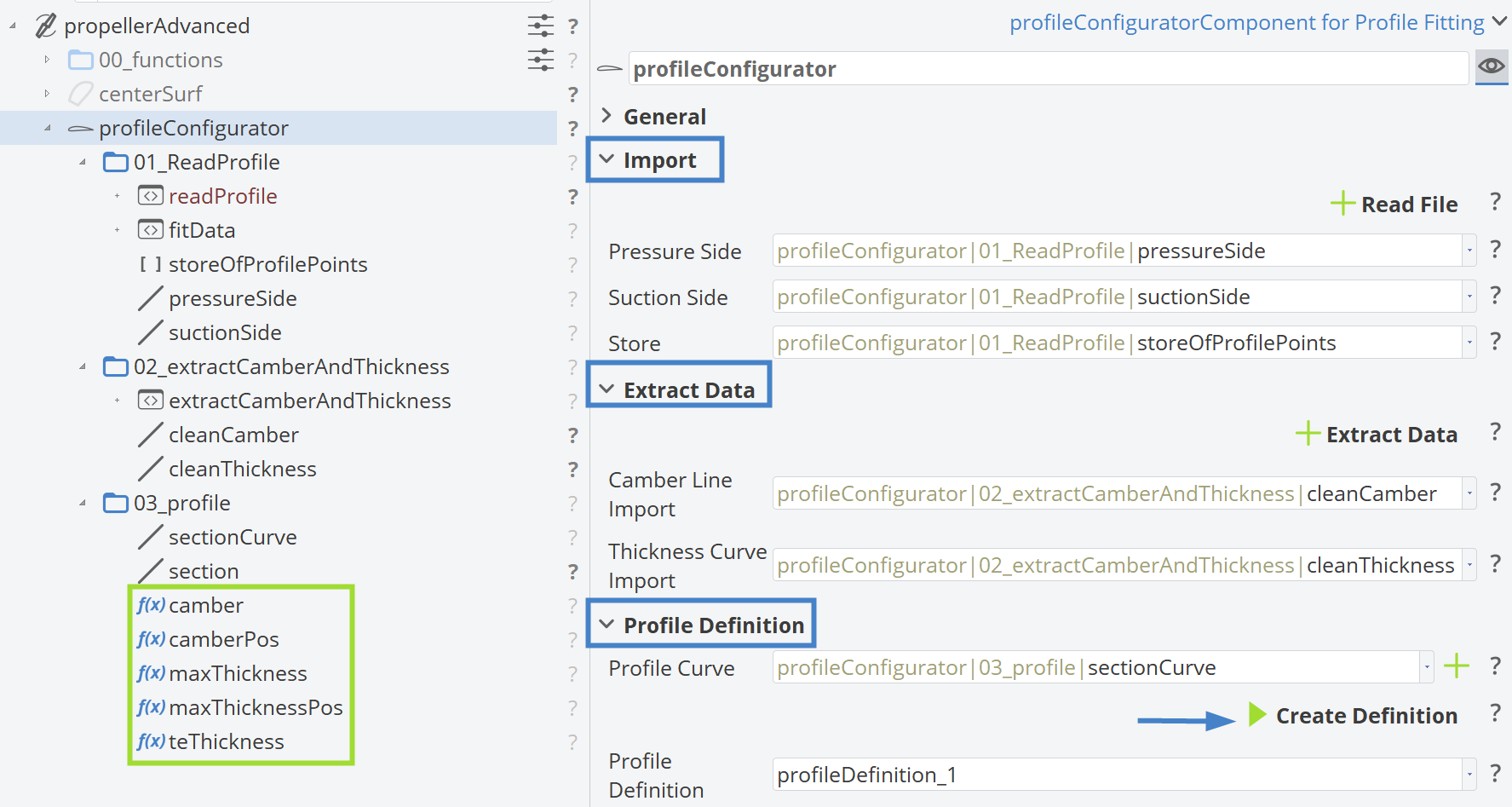
Finally, by pressing the Create Definition button, a Feature Definition is automatically generated for this parametrized profile based on the imported data, which is needed for the blade surface creation. This feature definition will later be used to create the FPropellerBlade, which is a specialized version of a MetaSurface designed specifically for blade geometry.

info

The camber and thickness are extracted from the imported file and parametrized to generate new shapes based on the imported profile geometry.

Blade Surface

In the Propeller Component GUI, continue by clicking the plus (+) button for the Blade Surface, then select Blade Surface again.
This action creates the following three objects:

• blade (type: FPropellerBlade)
• tipGap (type: FParameter)
• bladePrepared (type: FImageSurface)

By selecting the blade object (type FPropellerBlade), you will see the following GUI in the Object Editor:

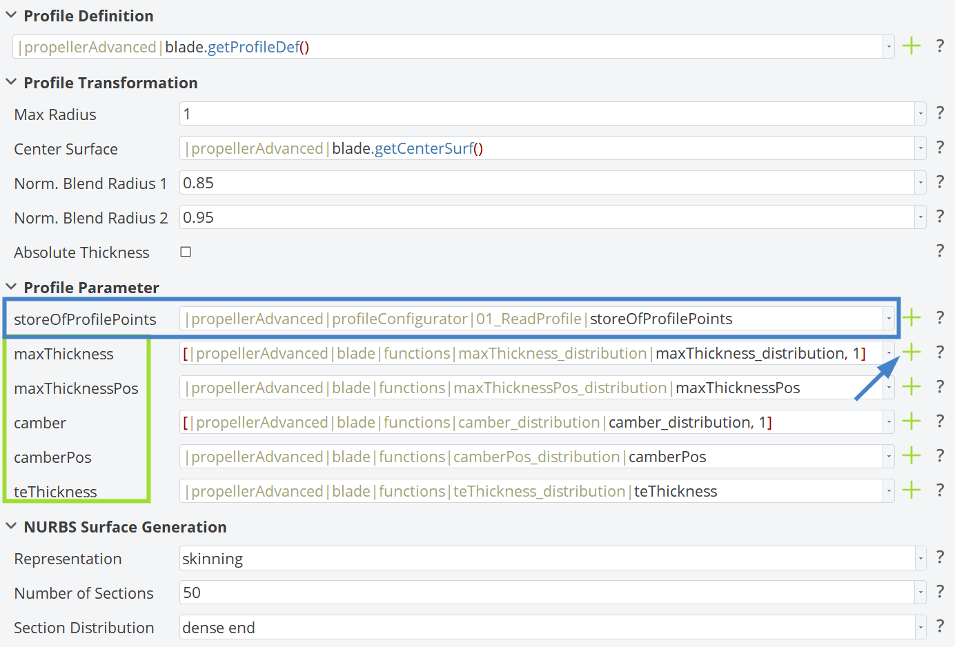
Here, you need to assign the correct input to storeOfProfilePoints, as shown in the image above.

In addition, distributions for several functions in the Profile Parameters section need to be defined, which will cover in the next section.

Distributions via B-Spline Curve

By clicking the plus (+) button, you can choose Distribution via B-Spline Curve for both the Camber and Thickness distributions.

The B-spline curve uses three control points:

• p00: The first point corresponds to the hub of the blade
  • Set the X-value of p00 to: |propellerAdvanced|00_functions|radiusHub
• p01: The second point corresponds to the mid-span of the blade
  • Set the X-value of p01 to: (|propellerAdvanced|00_functions|radiusHub + |propellerAdvanced|00_functions|radiusMax) / 2
• p02: The third point corresponds to the tip of the blade
  • Set the X-value of p02 to: |propellerAdvanced|00_functions|radiusMax

Camber

The Camber Distribution is controlled by the design variable camber_01.

• Set the bounds of camber_01 from 0.04 to 0.12, with a default value of 0.08.
  • Since p01 is a control point, this results in a peak camber of camber_01 in the curve.
• Convert camber_00 and camber_02 to parameters and set both to 0.
  • This creates a spanwise camber distribution that peaks at mid-span and reduces to zero at the root and tip.

Maximum Thickness

The Maximum Thickness Distribution controls the maximum thickness in the chordwise direction. It is driven by the design variable maxThickness_00.

• Set the range of maxThickness_00 from 0.15 to 0.25, with a default value of 0.2.
• Convert maxThickness_01 and maxThickness_02 to parameters and set them to: maxThickness_00 * 0.25
  • This provides maximum thickness near the root and gradually reduces toward the tip.

Constant Distributions

For Camber Position, Maximum Thickness Position and Trailing Edge Thickness, you can use constant values. Therefore, you do not need to use the plus (+) button for these.

Camber Position

• Create a sub-scope named "camberPos_distribution" under the functions scope.
• Define the design variable camberPos:
  • Set the Range from 0.3 to 0.4
  • Set the Default to: 0.35

Maximum Thickness Position

• Create a sub-scope named "maxThicknessPos_distribution" under the functions scope.
• Define the design variable maxThicknessPos:
  • Set the Range from 0.2 to 0.4
  • Set the Default to: 0.3

Trailing Edge Thickness

• Create a sub-scope named "teThickness_distribution" under the functions scope.
• Create the design variable with the name "teThickness":
  • Set the Range from 0.015 to 0.025
  • Set the Default to 0.02

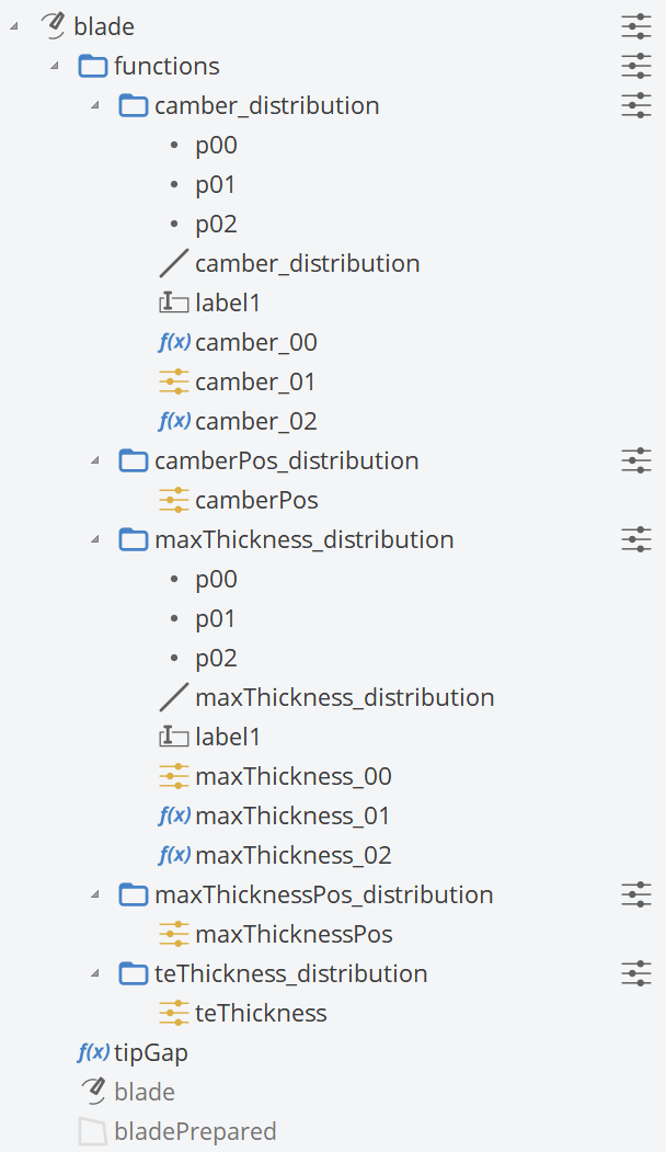
Blade Scope Structure

The figure below illustrates the scope structure once all distributions (both B-Spline and Constant) for the FPropellerBlade have been set up, including the corresponding design variables and parameters:

Tip Surface

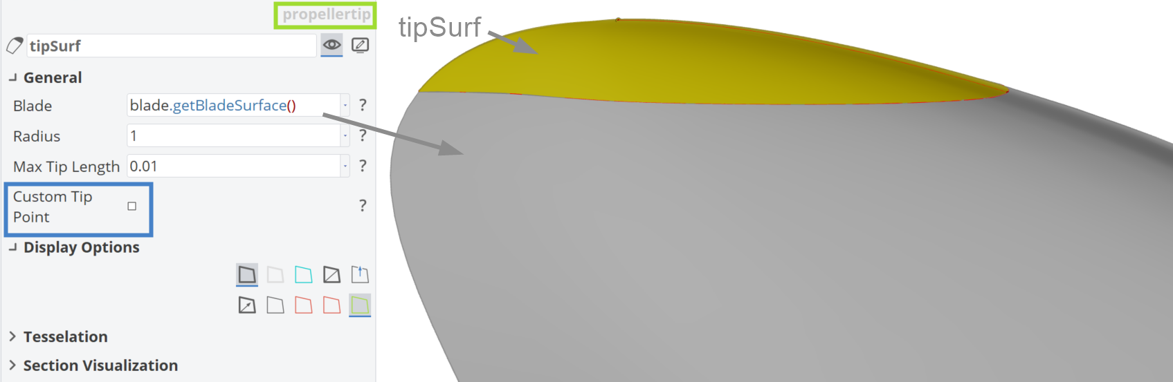
Here, the Tip Surface is created by clicking the plus button in the propeller component GUI. The following properties are automatically configured for this setup:

• Source: |propeller.getBladeSurface().getBladeSurface()
• Radius: 1
• Max Tip Length: 0.01

Below is a figure showing the tip region of the blade. The main part of the blade is depicted in gray , while the tip surface is highlighted in yellow color.

Propeller Solid

Following the creation of the blade and tip surfaces, the next step is to create a watertight, closed solid geometry.

• Click the plus button in the propeller component.
  • This will generate a bladeSolid component along with two design variables named "absPropellerRadius" and "NOB".
  • These correspond to the propeller radius and the number of blades (NOB).
• Set the range of absPropellerRadius from 100 to 5000 millimeters, with a default value of 2500.
• Keep the range of NOB from 3 to 5, with a default value of 4.
  • Set it as an integer design variable.
• Next, create a parameter under the bladeSolid component named "D".
  • This corresponds to the Diameter with the expression: D = absPropellerRadius * 2.

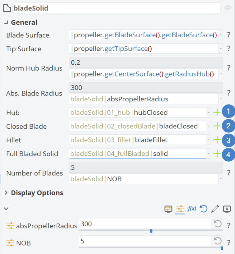
Steps for Propeller Solid Creation

The steps to complete these tasks are illustrated in the figure below.

Hub

By clicking the corresponding plus button in the bladeSolid GUI, you can create a hub BRep scaled to the propeller's radius. For this tutorial, the auto-configured hub from the workflow is sufficient.

Closed Blade

Afterward, you can create a Closed Blade as a BRep in a similar manner. This is achieved through an Operation: boolean|solid from intersections of a scaled version of the blade & tip surface to the propeller radius, combined with a scaled-down version (99%) of the hub geometry, named "hubSmall".

Variable Radius Fillet

Having BReps for the blade and the hub correspondingly, then we can move on to the Variable Fillet creation. A rule of thumb that we use for the fillet is to introduce fillet radius on the pressure side 2/3 times compared to max. profile thickness at the root and 1/3 times on the suction side accordingly. Also, the fillet should follow the thickness at the TE and the LE. Based on the aforementioned the following Parameters are defined:

• filletScalefactor = 10
• radiusLe = thicknessRoot / 10
• radiusSide1 = thicknessRoot / 3
• radiusSide2 = thicknessRoot * 2 / 3
• radiusTe = thicknessTE / 2
• thicknessRoot = |propellerAdvanced|00_functions|04_chord|chordRoot * |propellerAdvanced|blade|functions|maxThickness_distribution|maxThickness_00 * |propellerAdvanced|bladeSolid|D
• thicknessΤe = |propellerAdvanced|00_functions|04_chord|chordRoot * |propellerAdvanced|blade|functions|teThickness * |propellerAdvanced|bladeSolid|D

Full Bladed

The final step in the Propeller Solid process is to generate the complete propeller geometry, with all blades smoothly connected to the hub as a single BRep, as shown in the figure below.

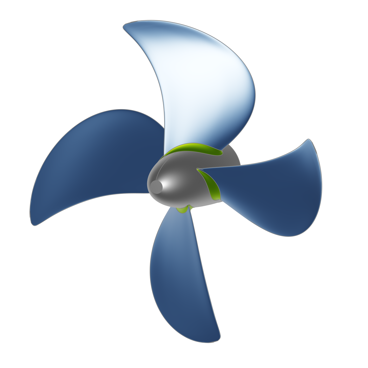
This tutorial demonstrates how to import profile data from external files into the Advanced Propeller Workflow in CAESES.
The imported profile can either be a well-known airfoil from literature or a custom-designed one.

Once imported, the profile data can be parametrized and used to generate a fully-parametric propeller model based on this profile.

This approach enables users to generalize the propeller design workflow in CAESES, making it more flexible and not limited to the predefined tools or profiles provided by default.

Final Setup

CAESES Project File

If you want to take a look at the finalized model you can find the resulting CAESES project file import-propeller-profiles.cdb here:

Load Final Model