Generic Blade Design
CAESES provides comprehensive functionality for designing different types of blades for various industries.
For marine propellers, CAESES offers a generic blade type that can be used in addition to the cylindrical transformation. The generic blade takes a feature definition (2D section parameterization) and transforms it into the 3D space. You can directly set rake, skew and pitch distributions.
The generic blade is also required if you want to export PFF files (Propeller Free Format): The generic blade is input for the propeller entity which finally provides the PFF export, including diameter and number of blades information. You can find both objects in the menu as follows:
- Model > Propeller > Generic Blade
- Model > Propeller > Propeller
In this tutorial, the Generic Blade entity is introduced, and as an example we will model a ship propeller. The Generic Blade transforms a given profile definition onto a cylindrical surface according to characteristic blade functions such as rake, skew and pitch.

For profile design, any CAESES curve type can be used. This also includes mathematical definitions (e.g. via Generic Curve). In this tutorial, a NACA curve will be utilized.
The radial functions of the blade are defined in a normalized system, which is the global XY-system of CAESES. Again, any kind of curve can be used to define functions. Typically, these functions are later on controlled by design variables in optimization processes.
The Generic Blade can serve as input for a Propeller entity, which is also briefly illustrated.
Prerequisites for this tutorial are the introductions to basic modeling and feature definitions.
Profile Definition
The user is free to design custom profiles using any curve type that is available in CAESES. Mathematical definitions such as customized airfoil definitions can also be set up for describing a profile. In this tutorial we will utilize a NACA profile that comes with CAESES, so that we can focus on the actual blade generation process. Profile definitions need to be provided in the XY-system of CAESES where the leading edge is expected to be located at the origin.
Let's get started and create a NACA profile:
-
Go to the Model workspace. Look for the Curves category and click on More and look for the curve NACA-4DS and click on it to create it. ( Model > CAD > Curves > More > NACA-4DS )
-
Set the name of the NACA-4DS curve to "profile".
-
Create parameters for the variable input values of the profile (chord length, thickness, camber, camber position) and set the names to "chord", "thickness", "camber" and "camberpos".
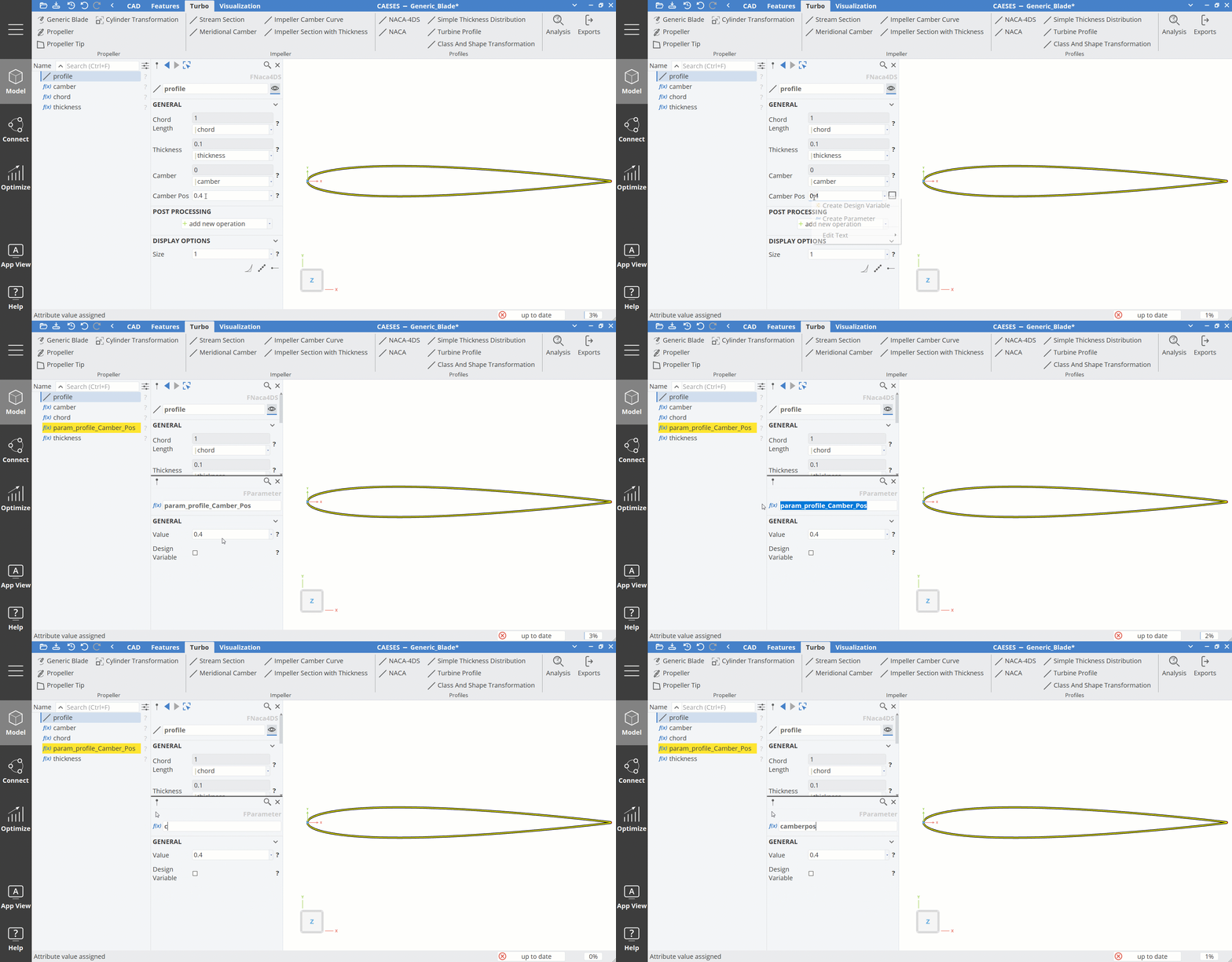
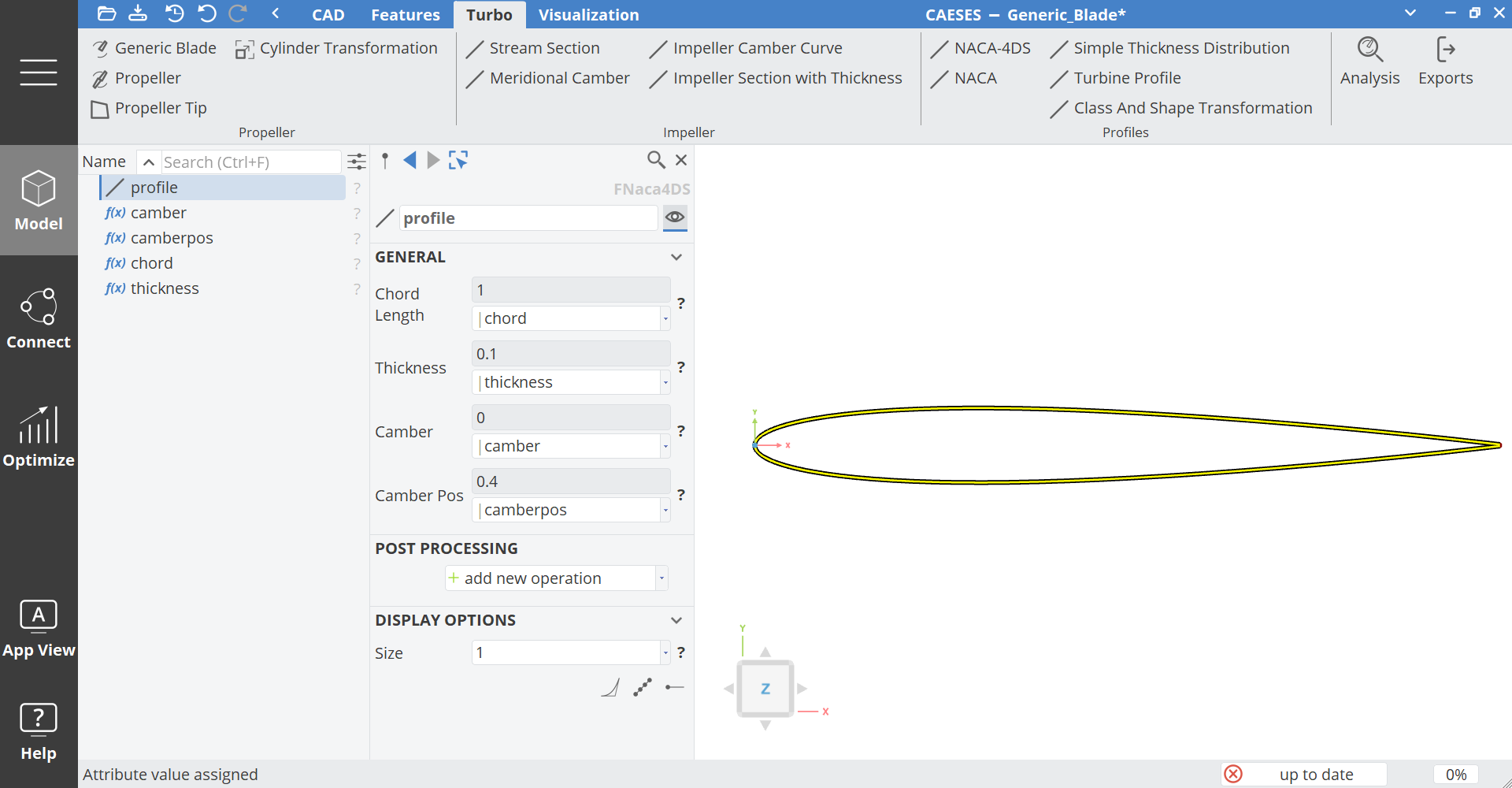
Your profile definition should now include parameters for all of the input values.
Feature Definition
Similar to Meta Surfaces, the Generic Blade entity is also based on Curve Engines. For this reason, we put the profile description into a feature definition, which will be used by the curve engine.
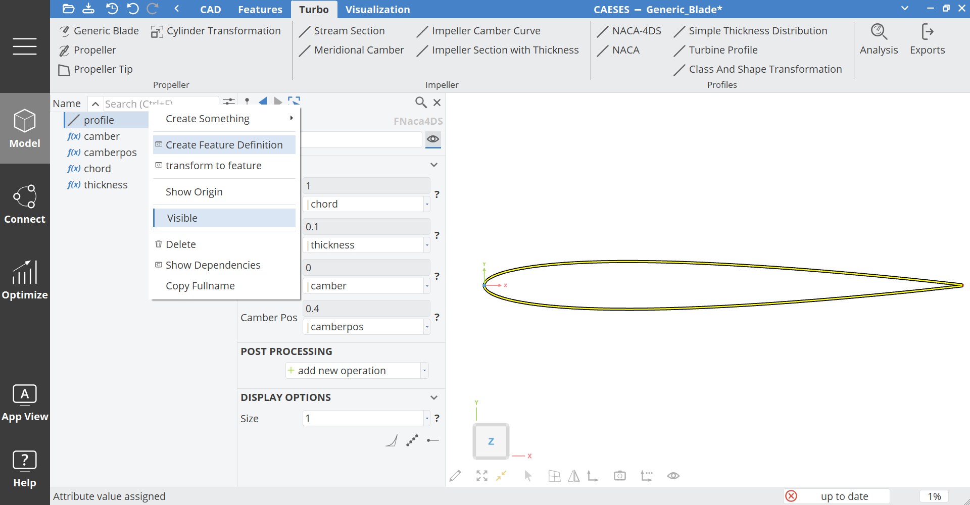
- Select profile, right-click and choose Create Feature Definition from the context menu.
- Edit the new Feature Definition and, set the definition's type name to "naca" (if you like, you can also use "naca4ds" etc.) in the General tab of the Feature Definition Editor.
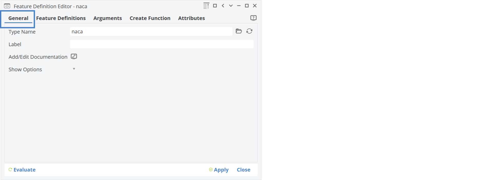
- Press the apply button and close the dialog.
The recently created feature can now be found in the Features Tab.
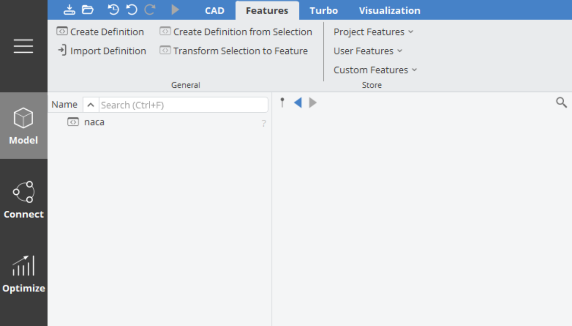
By this step, we have created a profile definition (naca) that can be used for surface creation. Keep in mind that the next steps of this tutorial are applicable to any other profile that is given as a Feature Definition. Therefore, the initial profile geometry from the first step is no longer needed:
- Select profile and the 4 parameters in the object tree (Model workspace > CAD tab) and delete them. Your object tree in the CAD tab should be empty afterwards, while the Features tab shows the naca Feature Definition.
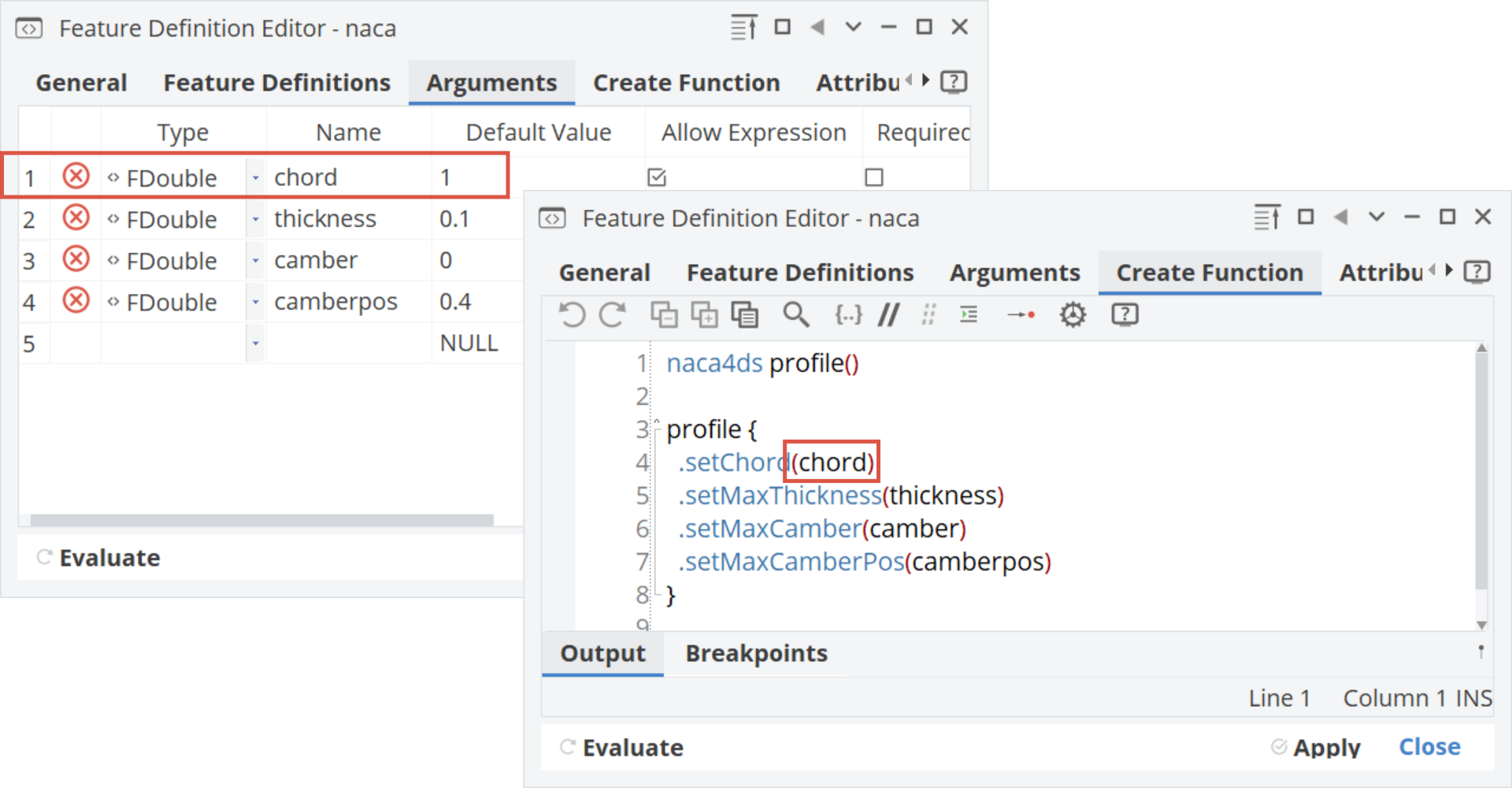
If you would like to use other custom profiles in combination with the generic blade, your feature definition always needs to have an input argument with name chord (type FDouble) as shown in the figure below. Otherwise, the surface generation won't work correctly.
So far we created a feature definition from a selection of objects, which is a convenient mechanism. Note that you can also start from scratch with a blank feature definition created from the ribbon in the Model workspace in the Features Tab by choosing Create Definition.
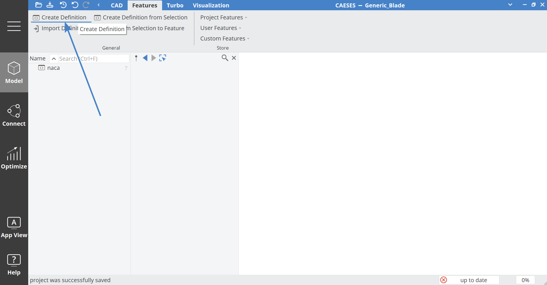
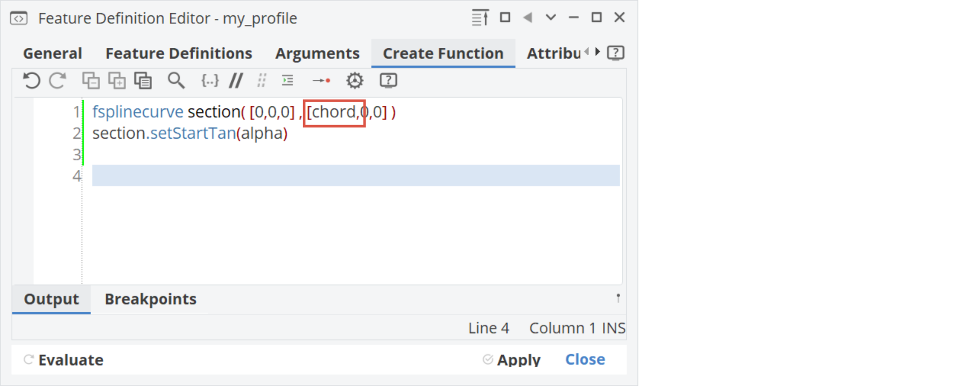
- Just type the definition of your custom profile curve as a sequence in the tab Create Function of the Feature Definition Editor. As mentioned above, make sure that you have at least an argument
chordwhich defines the length of the profile.
Curve Engine
Curve Engines connect the curve (i.e. 2D blade profile definition) with functions in a certain range to create flexible surfaces. For blade design, the range is given along the radius of the blade. We consider a normalized system for the profile and blade functions. The radius runs from the normalized hub radius (e.g. R=0.2) to the tip radius R=1. For a start, we will use constant values for the profile parameters. For instance, chord will not change in the radial direction. We will then create radial functions in a following step.
Let's create a Curve Engine, that we will use for our surface creation later. Curve Engines usually drive the Meta Surface creation (so that's where we will look for it).
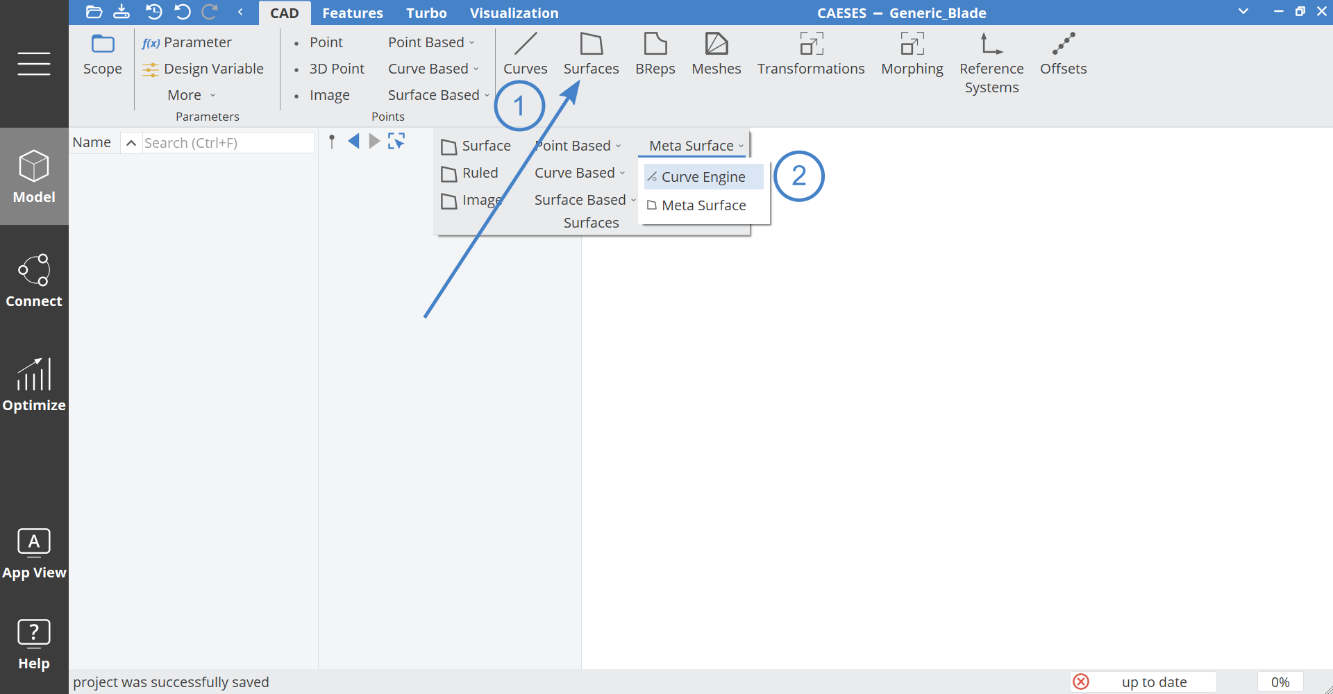
- Create a Curve Engine via Model workspace > CAD tab > Surfaces > Meta Surface > Curve Engine and name it "engine".
-
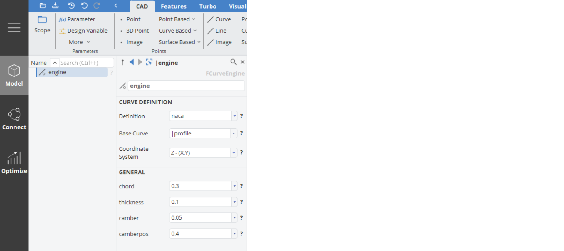
From the pull-down menu of Definition, choose naca in the object editor of engine.
-
Set initial constant values for chord, thickness, camber and camberpos according to the following screenshot:
Generic Blade
The Generic Blade requires at least one Curve Engine as input along with a (normalized) hub radius.
-
Create a Generic Blade in the Model workspace > Propeller tab in the Geometry category of the ribbon and name it "blade".
-
Choose engine from the pull-down menu of the blade attribute Curve Engine.
-
Introduce a parameter called "hubradius" for the hub radius of the blade (via right-click in the context menu).
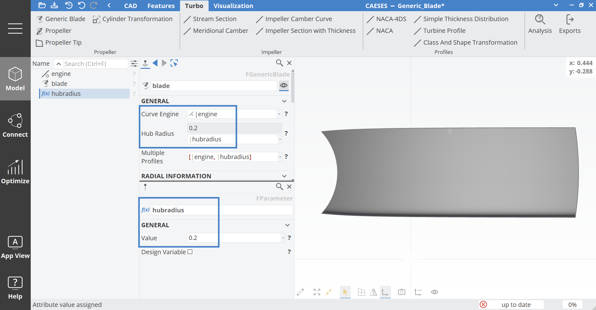
An initial blade is now visible in the 3D view. Play around with the parameter hubradius and the constant input values of engine.
Often only a single profile definition is applied in a blade generation process. If you want to have different profiles in the blade definition, insert them in the attribute Multiple Profiles according to the convention. You have to provide a list of Curve Engines along with their starting radius. See also the attribute documentation for more information by clicking on the question mark icon next to the field.
Radial Functions
We distinguish 2D profile parameters such as chord or camber position and 3D blade parameters such as rake, skew and pitch. For both kinds of parameters we introduce radial functions.
Radial Functions for 2D Profile Parameters
As an example, we start with chord:
-
Choose Model workspace > CAD tab > Curves > Point Based > Planar B-Spline.
-
In the dialog, set the name to "chord".
-
Set number of control vertices to
4. -
Set constant value to
0.3. -
Set start to
0.2(starting X-position of the function i.e. corresponds to "hubradius"). -
Press the Execute button.
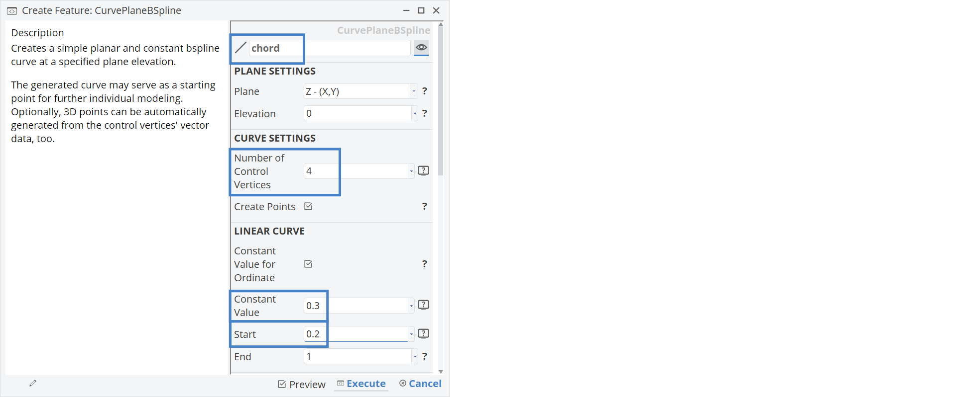
This creates an initially constant curve (i.e. a function for chord along the radius) in the XY-system. Let's organize our project structure slightly before we continue:
- Select the scope chord and create another scope via CAD tab > Scope (the scope chord is then put into the new scope). Rename the new scope scope1 to "functions".
You can use any CAESES curve type as a function, not just B-Spline curves.
Connect Radial Function to Curve Engine
Now we connect the chord function to the blade via the Curve Engine (remember: the Curve Engine is the input for the blade surface creation).
- Select engine and drag & drop the curve from scope chord into the corresponding attribute editor chord of the Curve Engine.
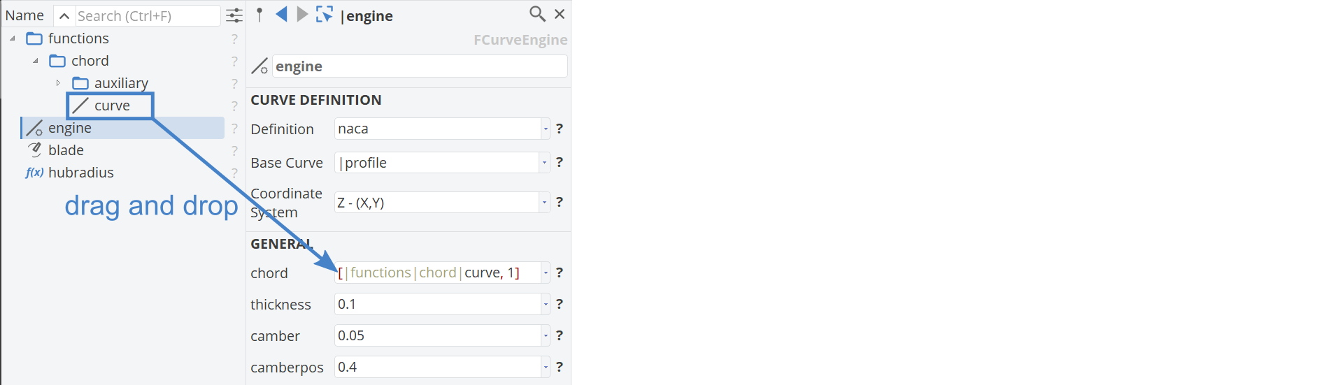
-
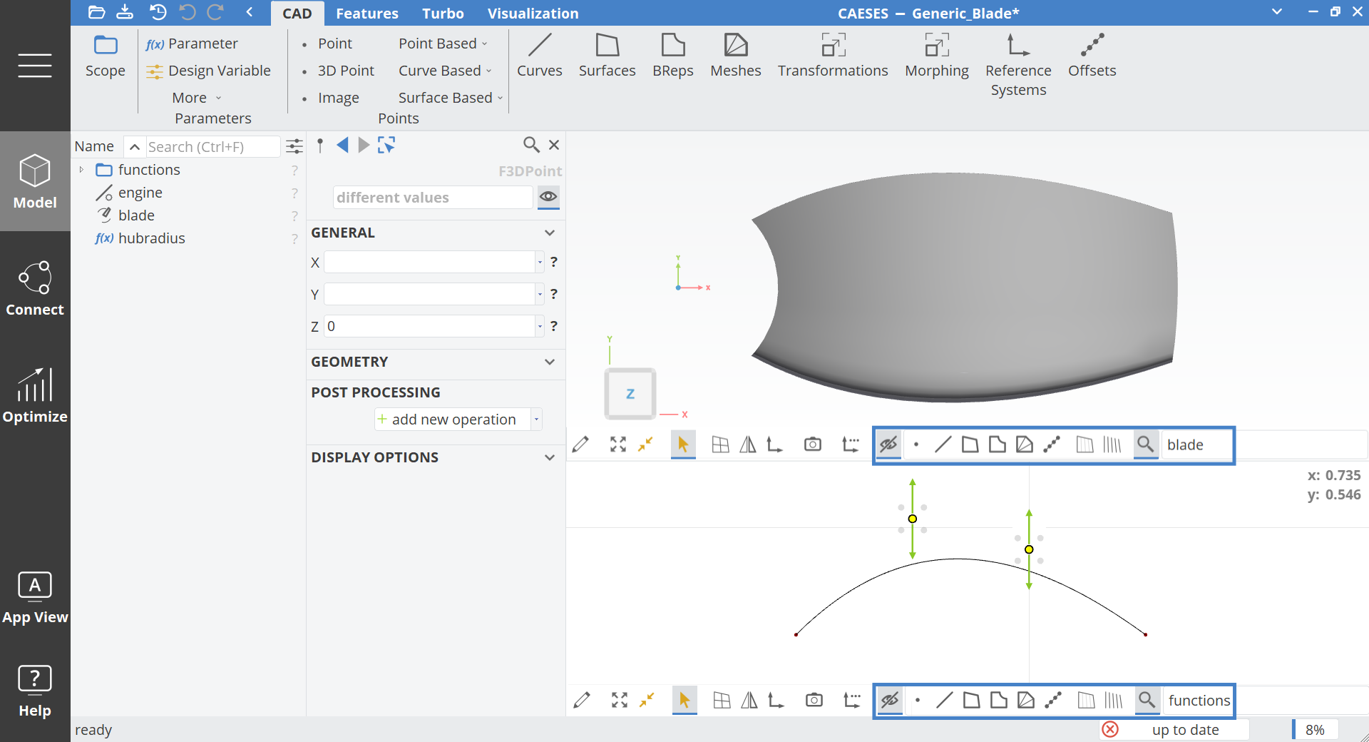
Open another window by choosing the Menu workspace > View tab > New > 2DFunctionsWindow.
-
See the screenshots below: Use the name filters of the two windows in order to filter only for the blade in 3DView, and only for the functions in 2DFunctionView.
-
Select some curve points of chord (from the subscope auxiliary or in the 3D window) and move them in the Y-direction to see how the chord length can be changed in radial direction.
Radial Functions for Other Profile Parameters
In order to keep it simple, we just copy & paste the chord function and adjust the curve points according to reasonable values for thickness, camber and camberpos.
-
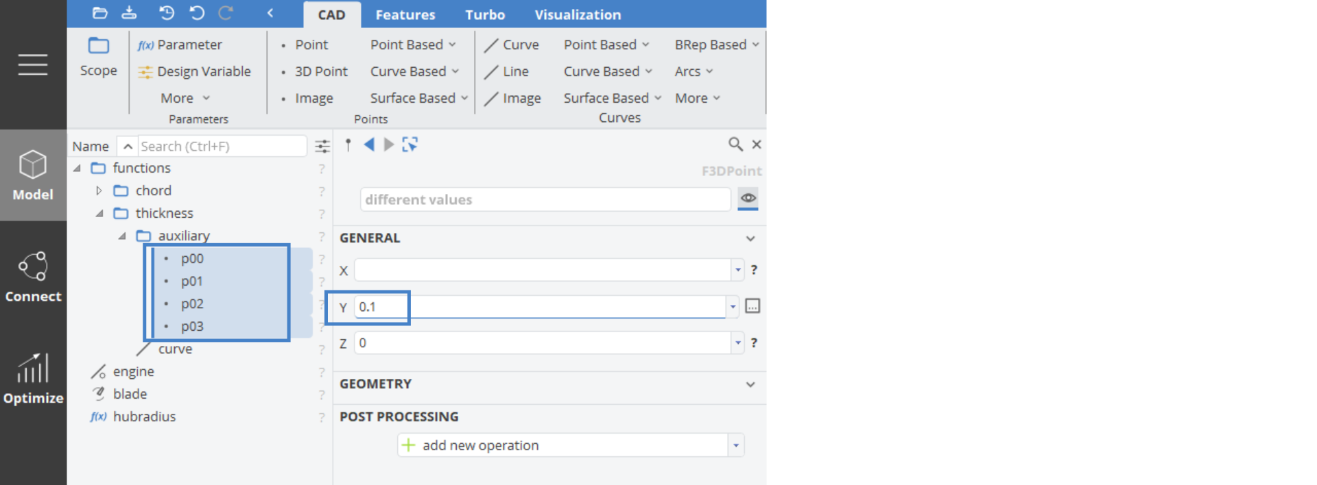
Select the scope chord (in scope functions) and copy & paste it.
-
Set the name of the new scope from chord01 to "thickness".
-
Select all four points of the thickness function in the object tree by holding the Ctrl button while you select them and set the Y-value to
0.1.
Let's repeat the previous step to connect the thickness function with the Curve Engine:
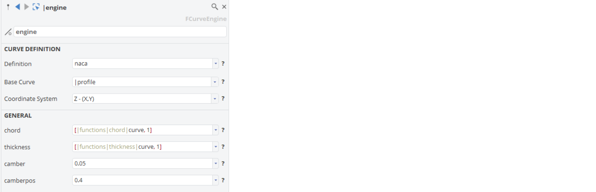
- Select the Curve Engine engine and drag & drop the thickness curve into the thickness attribute to connect it to the blade.
In the same manner, create radial functions for camber and camberpos.
-
For camber, set the Y-value of all four points initially to
0.05. -
For camberpos, set the Y-value of all four points initially to
0.4.
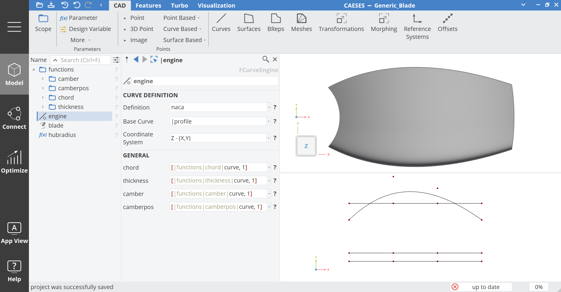
You can now change these functions interactively in the 3D window by moving their points in X- and Y-direction. Check out how the blade shape changes accordingly.
Note that the X-position of the first point (at x=0.2) needs to be untouched since this corresponds to our hub radius. This issue is addressed again in the section Hub Radius.
Radial Functions for 3D Blade Parameters
Functions for rake, skew and pitch can be set in the Generic Blade. Information about these parameters is given in the type documentation:
-
Select the blade object in the tree.
-
Click on the type icon of blade to show the documentation (see screenshot below)
-
Rake, skew and pitch are typical parameters used in propeller design. Read the documentation for the definitions (shown below).
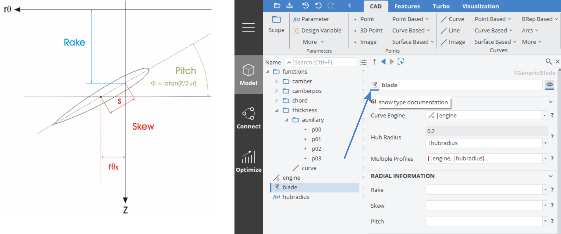
Function curves for these parameters are created as described in section Radial Functions for Other Profile Parameters, for instance, using an initially constant B-Spline Curve or via copy & paste of an existing function such as chord. Alternatively, use the smooth F-Spline Curve, an Interpolation Curve (interpolate point data) or the Generic Curve (for mathematical definitions). All curve types are given in the tab CAD in the category curves.
Examples for rake, skew and pitch are briefly given in the next step.
Examples for Rake, Skew and Pitch
Have a look at example functions for rake, skew and pitch. The following curves also stem from a copy & paste action of one of the existing curves (Planar B-Spline with 4 points). The values along the abscissa and the ordinate are displayed so that remodeling of such curves is easier.
Create a 2D Diagram in the Model workspace > Visualization tab to display a coordinate system and make the recreation of the curves easier. Drag and drop the coordinate system Diagram1 into the functions scope to only make it visible in the lower 2D Functions Window.
-
Let's organize the object tree a little bit. Mark the scopes camber, camberpos, chord and thickness and create a new scope. Name it "2D_profile".
-
Create another scope and drag and drop it into the functions scope. Name it "3D_shape".
-
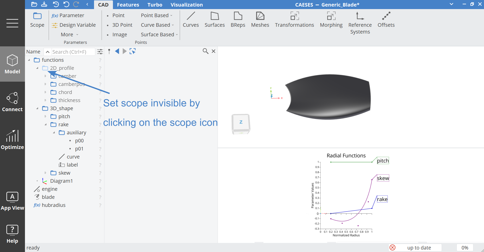
Set the 2D_profile scope invisible for now (by clicking on the blue scope icon in the object tree) to focus on the creation on the new blade functions.
-
Copy and paste an existing scope, e.g. camber into the 3D_shape scope and change the values of the points according to the screenshot below. You can simply drag the points to the desired position.
-
You can add or remove auxiliary points for each function curve. Simply create new 3D Points, put them in the corresponding auxiliary scope and set them for the B-Spline Curve.
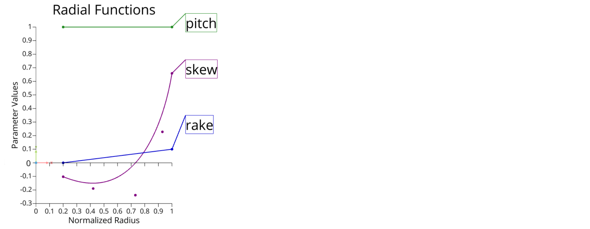
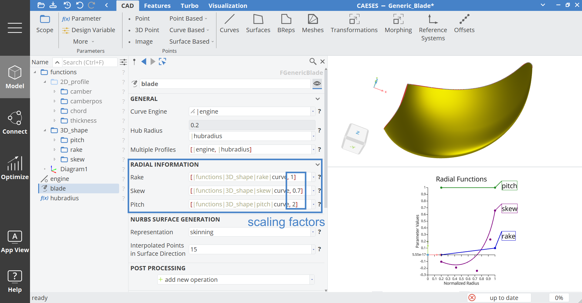
- Set these three curves at the blade (category Radial Information), see the screenshot below.
We can also use a scaling factor for each function. Hence, these curves can still be designed in a normalized system (e.g. convenient visualization) but the ordinate values get scaled internally. Replace the default value of 1 (no scaling) with a new value for the factor. Note that this might also be a separate parameter that can be controlled. The function values are then automatically scaled by this value during blade surface generation. Try to change these values and watch the surface generation.
Colors and Labels
Colors
So far, an initial blade has been generated and radial functions control the shape. For convenience, it is often useful to assign different colors and labels to the functions in order to manipulate them more easily.
Assign different colors to the functions:
-
Select the curve functions and set a color in the Display Options category of the object editor.
-
Mark all points in the auxiliary scope and give them the same color as the curve.
Labels
To assign labels for the functions:
-
Choose Model > Visualization > Label and move the new label into the function scope.
-
Set a position for instance, drag & drop the last point of the curve into the position attribute.
-
Set a text, such as "skew".
-
Set a font scaling of
0.1. -
Configure background settings (e.g. draw frame filled etc.).
Hub Radius
Usually, the hub radius is fixed and will not change. However, for a proper parametric model, the hub radius might also be a parameter that can be changed: All functions then simply follow i.e. they change their range according to the new hub radius. So far, the parameter hubradius has been set for the blade but not for the functions which we change in this step:
-
Set the 2D_profile scope visible by clicking on the icon in the object tree. The function curves should be visible in the lower window afterwards.
-
Select the first curve point of all seven functions (this can also be done all at once using Ctrl, or in the 3D window, select all first points with a single selection).
-
Drag & drop the parameter hubradius into the X-coordinate.
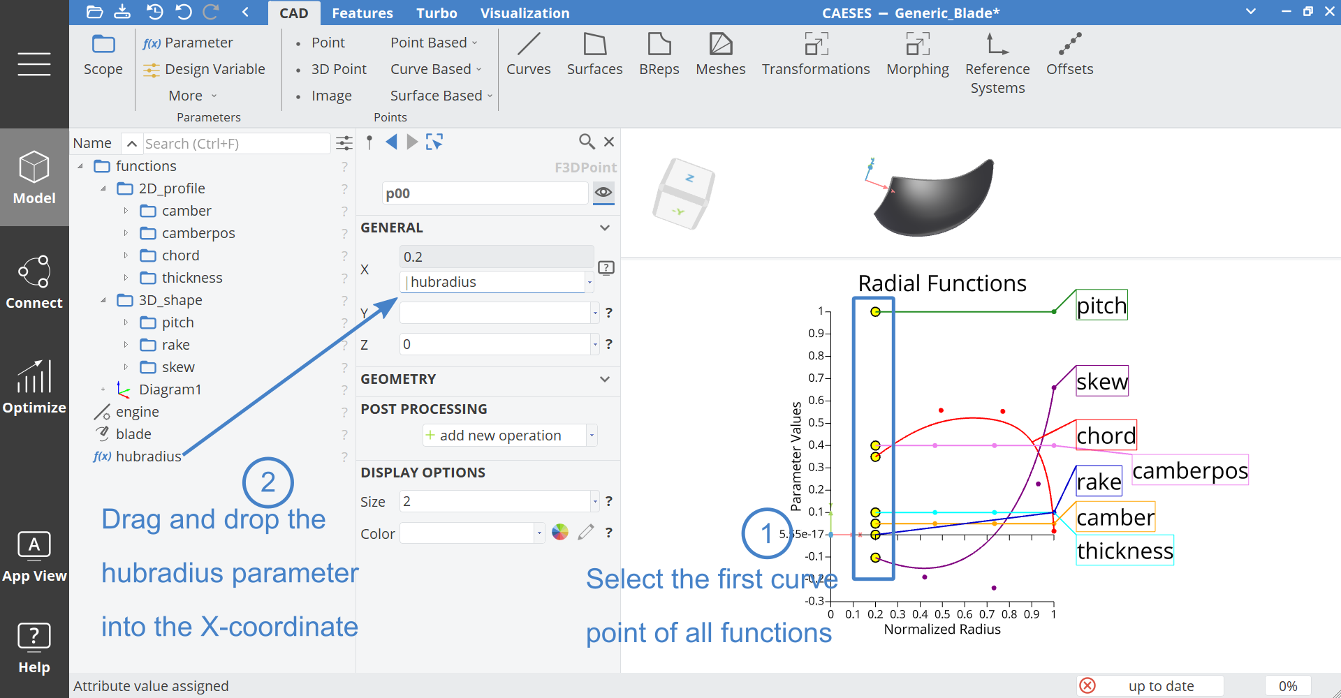
Previously, only the discrete value of the hub radius (0.2) was used to set the X-coordinate of the first point. In this step the parameter hubradius is used to control the X-coordinate of all functions.
- Try values for hubradius such as
0.15or0.25.
Make sure that the X-coordinate of the first point is smaller or equal than the second point. For instance, large values of hubradius will result in an invalid function since the other curve points will not adapt automatically (they are not dependent on hubradius so the X-coordinate of the first point can get greater than the X-coordinates of the other points).
Propeller
The blade has a normalized outer radius of 1. The propeller entity allows scaling of the blade to the real dimensions.
-
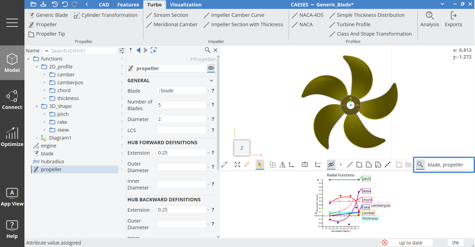
Go to Model > Propeller tab > Geometry category > Propeller and create a propeller object.
-
From the pull-down menu of the attribute Blade, choose our blade.
-
Set number of blades (attribute NOB) to
5.
If you cannot see the propeller, check the name filter at the bottom of the 3D view. You could also type "propeller" in the name filter section so that your filter states "blade, propeller" to see the propeller geometry.
Conclusion
In this tutorial the generic blade entity is presented and a simple blade surface is generated that can be used in a PFF file (propeller free format). Similar to Meta Surfaces, the blade is also based on a curve definition that is connected to user-defined function curves via the Curve Engine.
The blade surface can further be fine-tuned by using its NURBS attributes. See also the Meta Surface introductory tutorial for more information.
There are additional options available for the blade -- just click on the different categories to view them (for instance, the category Profile View Options).
The generic blade conveniently comes with a set of blade-related attributes and options such as rake, skew, pitch and profile view options etc.
In case you need a closed propeller model, follow the advanced propeller workflow tutorial for a full propeller setup including a closed geometry, fillets and a flow domain.
A more generalized way of generating a blade surface can be realized with Meta Surfaces in combination with a Cylindrical Transformation. Such a design process is demonstrated in the Cylindrical Transformation tutorial.
For turbomachinery blades, the Turbomachine Workflow guides you through the creation of compressors, turbines, pumps or fans and allows mapping of 2D profiles onto arbitrary stream surfaces i.e. not just cylindrical stream surfaces.
CAESES Project File
If you want to take a look at the finalized parametric model and to see how the radial functions were modeled for this tutorial you can find the resulting CAESES project file generic-blade.cdb here: