Optimization Methods
CAESES provides a set of strategies for single- and multi-objective optimization. There are also response surface methods available that allow you to run optimizations on surrogate models.
You find all design engines in Optimize > Optimization > Design Space Exploration
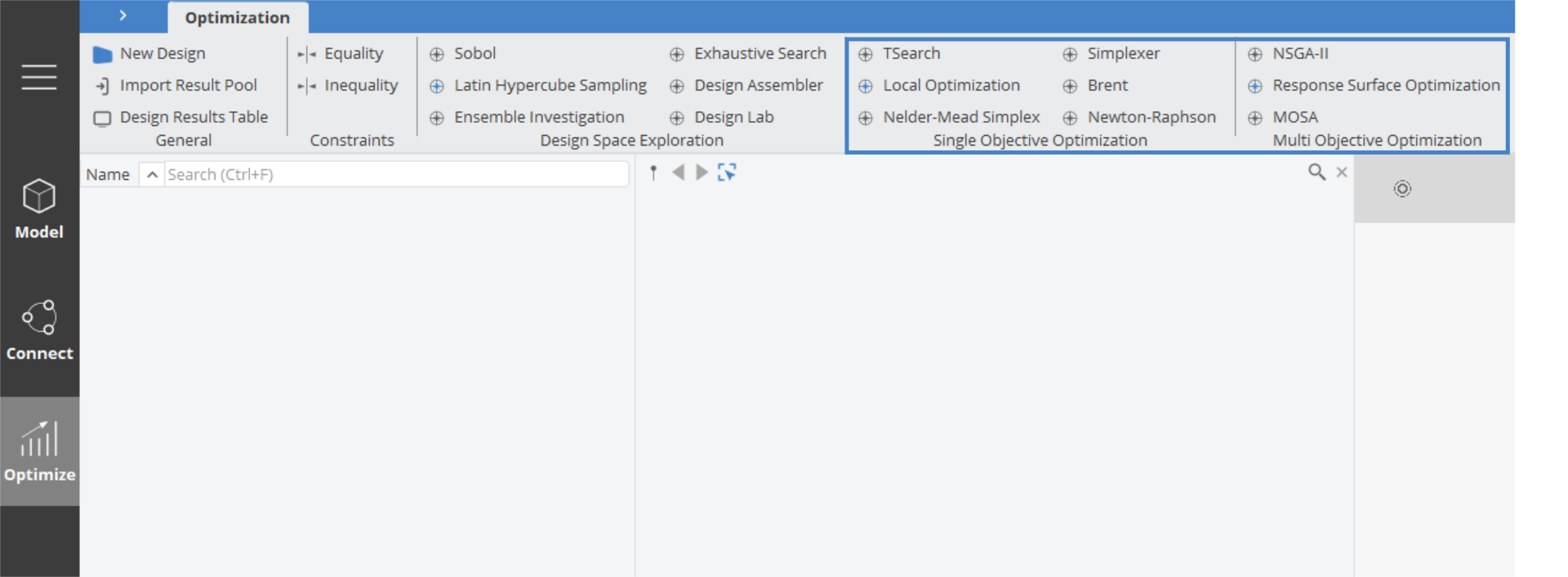
Single Objective Optimization
You find these design engines in Optimize > Optimization > Single Objective Optimization
TSearch
The Tangent Search Method (TSearch) promises to be a reliable solver for small scaled, single-objective optimizations problems with inequality constraints. The major features of the Tangent Search Method are to detect a descent search direction in the solution space, to ensure fast improvement in the promising search direction, and to keep the search in the feasible domain.
Within the permissible solution space the Direct Search Method is applied which consists of exploratory moves that start from a so-called base point along the variable axes followed by global moves in the descent search direction found in a successful exploratory moves. If a constraint bound is approached a tangent move in hyperspace is conducted tangential to the constraint either to keep the search in the feasible domain or to bring it back to the feasible domain.
The method is capable of detecting a local minimum of the solution space which is of dimension N * V according to the number of free variables. A descent search direction is determined by at most 2 * N * V function evaluations. Free variables are subject to explicit bounds, i.e. a lower and an upper bound. Satisfactory results are usually obtained by setting the initial step size to be 5% to 10% of the respective variable range. The minimum step size is about 5% to 10% of the initial step size.
If more than just one objective is given, a weighted sum is taken into account.
Reliable optimizer for local optimization problems.
The Tangent Search Method is a reliable optimization algorithm which works well for many different tasks. It is often used in combination with a Sobol run where the best candidates of a Sobol run is taken as starting design for the Tangent Search.
Local Optimization (Dakota)
Gradient-free local optimization strategy. Recommended method to further optimize an existing good design.
Depending on the problem, it will perform slightly better than the TSearch.
Nelder-Mead Simplex
Similar to search methods the Downhill Simplex Method of Nelder and Mead only requires function evaluations, not derivatives of the optimization function. It is a single-objective algorithm that can involve inequality constraints.
A simplex is the geometrical figure consisting, in N dimensions, of N+1 points (or vertices) and their interconnecting lines, polygonal faces. In two dimensions, a simplex is a triangle. In three dimensions it is a tetrahedron and so forth. It is assumed that the simplex in non-degenerated, which means that no edge of the simplex is parallel to any other in N-dimensional space, e.g. a triangle does not have parallel sides. The simplex moves in the design space, seeking for the (local, at least) minimum. The moving operators are reflection, expansion, and contraction.
For N-dimensional minimization, the downhill simplex method must be started with N+1 points, defining an initial simplex. Usually, the initial guess may be N+1 promising design candidates which are selected from a previous DoE (Design of Experiments) sequence (e.g. a Sobol sequence). The algorithm is then supposed to make its own way through the design space.
A robust but not super efficient optimizer that can include inequality constraints.
The Downhill Simplex Method is not very efficient in terms of the number of function evaluations that it requires. However, the method may frequently be the best method to use if one needs to "get something working quickly" for a problem whose computational burden is comparatively small. The Downhill Simplex Method is known to be a robust single-objective optimizer.
Simplexer
The Simplexer uses repetitive linearization of a non-linear objective function and constraints to be able to solve them with the linear Simplex method.
The traditional two-phase Simplex method is used to solve linear problems subject to one objective function and one or multiple equalities or inequalities. The method is restricted to solving problems in which the design variables are non-negative. Phase one and two of this Simplex algorithm consist of moving the initial guess into the feasible domain (if needed), and finding the minimum objective value in the feasible domain, respectively.
The Simplexer helps you to find an approximate minimum solution in highly-constrained design spaces.
The Simplexer can be applied to a minimization problem with one objective function and non-negative design variables. It linearizes the objective function and constraints around the initial guess, and finds the minimum for the linearized problem. The Simplexer then proceeds to linearize the objective function and constraints around this solution, to find a solution closer to the minimum of the non-linear problem. As soon as the solution does not change significantly during a new minimization step, the solution is considered converged and a minimum is found.
Things to keep in mind while using this design engine:
- Since phase one of the Simplex method moves the initial guess into the feasible domain, an option is added to perform only this step (without looking for the minimum). It may help find a feasible solution if it is difficult to determine manually.
- Linearizing constraints has consequences: it is possible that a linearized constraint is satisfied by the solution found, but the non-linear constraint it not.
- This method finds local minima, and solutions may differ based on initial guess.
- By default, this method enforces design variable bounds by adding them as inequality constraints. This option can be turned off. However if the solution causes design variables to be out of bounds, their values will be forced back into bounds (changing the solution).
Brent
This algorithm uses Brent's one-dimensional minimization algorithm to locate the minimum of the functional value within the bounds of a single free variable.
Basically, Brent's method applies a Golden Section Search whenever the objective function is "not cooperative" and switches to an iterative parabolic interpolation scheme when the function allows it.
Given a function f(x), and given a bracketing triplet of abscissa points a, b, c such that b is between a and c, and f(b) is less than both f(a) and f(c), this algorithm iteratively isolates the minimum to a fractional precision of about the given tolerance using Brent's method.
Use the Brent for simple optimization tasks with one free design variable.
Typically, this algorithm is not used for common optimization tasks where simulation is involved. It can vary only one variable. Similar to the Newton Raphson, the Brent engine is rather used for solving geometric optimization tasks such as finding the shortest distance to a point etc., mostly in feature definitions.
Newton Raphson
The Newton-Raphson Method belongs to the class of gradient methods which rely on a local quadratic approximation of the objective function. It is a single-objective algorithm. The approximation is achieved by second order partial derivatives, e.g. via the Hessian matrix of the objective function. The algorithm is an iterative one.
Second order methods like the Newton-Raphson algorithm are very efficient for nearly quadratic problems although the effort for accurately computing the higher derivatives in the Hessian matrix might abolish (depending on the problem at hand) the advantage of the method over other gradient methods. A very efficient means of convergence is given if the initial guess or starting point is sufficiently good (start point sensitive).
Great and fast for small optimization tasks that have a quadratic characteristic. Allows you to consider equality constraints.
Typically, this algorithm is not used for complex optimization tasks. Similar to the Brent, it is quite powerful for rather geometric or mathematical optimization tasks where e.g. a squared distance needs to be minimized etc. It is often used in feature definitions.
One Step Steepest Descent
The One Step Steepest Descent is a very simple optimization algorithm for small scaled, single-objective optimization problems. The main advantage of this algorithm is the very low number of evaluations required to find a first improvement.
In the first stage, the n-dimensional gradient of the objective function is determined by performing n+1 evaluations, with n being the number of free variables considered.
Once the gradient is determined, a one dimensional search for the optimum in the direction of the steepest gradient is performed. The step size for the initial step is guessed based on the derivatives from phase 1. The maximum number of steps is controlled using the Gradient Search Steps value. It should be noted that due to the simplicity of the approach (one dimensional search), the resulting design cannot be considered a fully optimized design.
A quick way to find good improvements with a low number of evaluations needed.
Multi Objective Optimization
NSGA-II
The NSGA-II design engine implements the famous non-dominated sorting based multi-objective evolutionary algorithm. It requires settings for the number of generations, the population size, the mutation probability as well as the crossover probability.
The crossover probability affects the process of mixing up the genes of the parents while creating a child, e.g. if this value is zero the genes of one single-parent are just copied to the child without crossing w.r.t. the other parent.
This algorithm is a good choice for optimization problems where several - often conflicting - objectives need to be minimized (i.e. not just one objective). It can also consider inequality constraints. Alternatively, you can also choose the MOSA.
As an alternative and for users of the advanced optimization add-on, the Global Optimization method from the Dakota engine is recommended.
Response Surface Optimization (Dakota)
Advanced OptThis functionality requires the Advanced Opt add-on to be enabled.In this method, a MOGA is conducted on a response surface that is iteratively built-up. For the initial response surface, data from a previous run (e.g. a sensitivity analysis) can be optionally considered. The best designs of each MOGA run get evaluated and are added to the response surface. This updates and improves the response surface model in each iteration. With this approach, the method tries to reduce the number of expensive evaluations such as CFD runs. Suitable for single- and multi-objective problems.
This is the most efficient method of CAESES for multi-objective problems, and works robustly for many engineering tasks. Check the Dakota Tutorial for more information.
Some comments about the attributes:
The entry “Solutions Considered” defines how many designs from the Pareto frontier are picked and evaluated after each iteration. For instance, 10 corresponds to 10 CFD evaluations after each iteration - if there are 10 or more than 10 Pareto solutions.
If you set “Initial Samples” to 0, then no sampling takes place for building the initial response surface. Instead, you can choose the designs from the previous sensitivity analysis (or from any other run). If you set a number that is non-zero, a Latin Hypercube
Sampling is triggered in the first stage to create samples that are used for the response surface.
The number of initial samples needs to be at least ~5 times the number of design variables.
MOSA
Dominance-Based Multi-Objective Simulated Annealing (MOSA) is an extended version of the common single-objective simulated annealing (SA) method. The idea behind SA is an analogy with thermodynamics where a slowly cooling metal adopts a low-energy crystalline state. Unlike this, if a liquid metal is cooled quickly it does not reach this minimum state - which follows the so-called Boltzmann probability distribution.
This specific design engine generates a number of samples (which is called duration) for each epoch using a fixed system temperature. After finishing an epoch the temperature is lowered and new samples are created again and so on. A sample is set by perturbing only one design variable where this variable is chosen at random and perturbed by means of a Laplacian distribution. Here, the attribute sigma is the scaling factor and sets the magnitude of the perturbation.
Choose this engine if you have several objectives (and not just one) that need to be minimized. The MOSA also considers inequality constraints. Alternatively, you can also choose the NSGA-II engine which solves the same optimization task.
Similar to the NSGA-II, use the "Global Optimization" method from the Dakota engine if available.
More Dakota Strategies
Advanced OptThis functionality requires the Advanced Opt add-on to be enabled.The advanced add-on of CAESES comes with an interface for Dakota, the optimization toolkit from Sandia National Labs. Dakota is a comprehensive library of numerical algorithms which can be easily accessed through the GUI of CAESES. There is no additional installation required, it runs out of the box.
Besides the capability to run any strategy of the toolkit, CAESES gives you a selection of methods that can be run with a single click. There is no expertise required about Dakota to run it.
Check the Dakota Tutorial for more information and to learn how to set up an optimization using the Dakota toolkit.
Local Optimization Multi-Start (Dakota)
Advanced OptThis functionality requires the Advanced Opt add-on to be enabled.This strategy allows you to run several local optimizations from different starting points at the same time. The starting points are randomly generated. For each local search, a gradient-free strategy is applied.
Great to check several local minima at the same time.
Global Optimization (Dakota)
Advanced OptThis functionality requires the Advanced Opt add-on to be enabled.Single-/Multi-Objective Genetic Algorithm (MOGA). This strategy is recommended for global optimization tasks. The initial population size as well as the number of generations can be set by the user. Recycling of existing designs from other runs for the first generation is also possible.
Note that genetic algorithms need many evaluations. This makes this method suitable only for problems where the evaluation (analysis) is not too expensive.
State-Of-The-Art optimizer for multi-objective problems and highly recommended for global optimization tasks.
Design Space Dimensionality Reduction
The design space dimensionality reduction method is practically not an optimization algorithm itself, but rather helps to reduce the number of free design variables that are used for the optimization procedure, while only sacrificing a small portion of the model's variability.
Often sophisticated parametric models are set up with a large number of design variables, that make the optimization task resource-intensive, time consuming and expensive. The higher a system’s degree-of-freedom (number of free design variables) the more simulations are usually needed to understand the system and to find improved designs. Faster optimizations come from intelligently reducing the degrees-of-freedom (free design variables) and, as a consequence, cutting down the necessary number of simulation runs.
The dimensionality reduction method used in CAESES, introduces so called Principal Parameters, by means of a Principal Component Analysis (PCA). Therefore the shape modifications undertaken by the free design variables are analyzed and converted into the Principal Parameters. Usually highly complex models with more than 20 design variables can be reduced to as little as five principal parameters while retaining more than 95% of the model's variability.
This method only takes geometrical design variables into account that influence the shape of the model.
Once the dimensionality reduction is set up, it can be used in combination with any optimization strategy. When an optimization is undertaken with a dimensionality reduction model as a basis for shape modifications, the Principal Parameters determine every new shape variant. In order to ensure the model's quality each shape defined by the principal parameters is transformed back to the original design variables automatically.
Principal Parameters
The Principal Parameters define every new shape when a Dimensionality Reduction method is used in a Design-of-Experiment (DoE) or optimization method.
Principal Parameters are sorted by their influence on the shape modification. This means that the first Principal Parameter is the most significant one in terms of capturing the greatest amount of variance. The second Principal Parameter is the second most important dimension, etc. Therefore the last Principal Component's influence is vanishing small and does not contribute much to the model's shape modifications. This ensures capturing the largest spread of modifications with the first few Principal Components.
In the dimensionality reduction object the number of principal parameters can be set, that are used for the optimization. In order to facilitate the decision of how many principal parameters should be used, the percentage of retained variability is displayed.
See the tutorial on dimensionality reduction to get an introduction on how it can be used.