Axial Turbomachine Workflow in CAESES

TurboThis functionality requires the Turbo add-on to be enabled. 5.2.0This functionality requires CAESES version 5.2.0 or later.

This chapter proposes a step-by-step guide to design an axial turbomachine in CAESES with the help of the Turbomachine Workflow.

For radial machines such as centrifugal pumps and compressors, see the Radial Turbomachine Workflow. For volute and housing geometry, see Volute Design.

Related tutorials: Axial Compressor · Turbo Analysis Tools · Blade Profile Design

Overview

CAESES offers capabilities for modeling and shape optimization of any type of blade, e.g. for pumps, fans, turbochargers, aero engines and propellers. Inside the turbo section, a newly implemented design workflow was introduced called Turbo Machine Workflow, which is a step-by-step guide to lead you through the modeling process of complex turbo machine components and offer you a variety of design options to find your optimal tailored parametric design, which can then e.g. be optimized in a simulation driven optimization.

Turbomachine Workflow

The wizard-like approach supports beginners and advanced turbomachine designers in selecting and using machine type dependent features available within the add-on TurboThis functionality requires the Turbo add-on to be enabled., keeping the project structure clean and organized, and making the modeling process faster. It is also possible to only use the structure of the workflow and implement your fully customized definitions for the meridional contours, airfoils or 3-dimensional airfoil transformations.

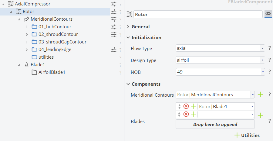Turbomachine Workflow in CAESES

The turbomachine workflow provides both an extensive selection of dedicated design components, and a step-by-step guide through the geometrical modeling process of a fully-parametric turbomachine design. After setting the machine (compressor, turbine, pump or fan) and the flow type (centrifugal/radial or axial), the workflow streamlines the creation of every necessary geometry object and parameter, to help you create a powerful and flexible parametric model in less than half an hour.

The overall structure for designing an axial turbomachine component inside the Turbo Machine Workflow in CAESES is shown in the following image.

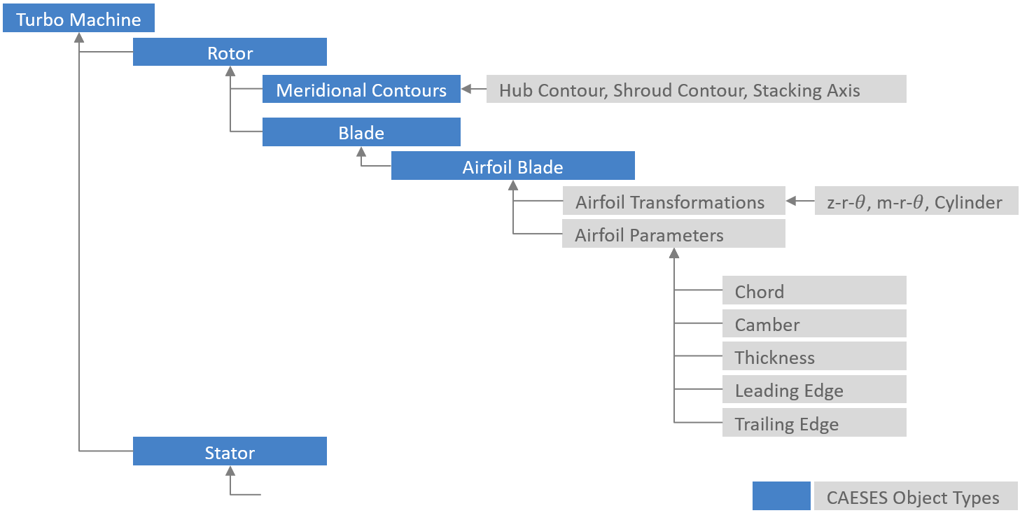
Turbo Machine Workflow structure for axial turbomachine components

Let's start to model a parametric axial machine inside the Turbo Machine Workflow.

Step 1 | Turbo Machine

To start your parametric turbo machine design create the TurboMachine object by clicking on the Model workspace > Turbo tab > Turbo > Turbo Machine workflow.

In the drop down menu for the Machine Type choose the machine type you would like to model. The machine type will be used internally to suggest type specific objects, features, and commands in the design workflow.

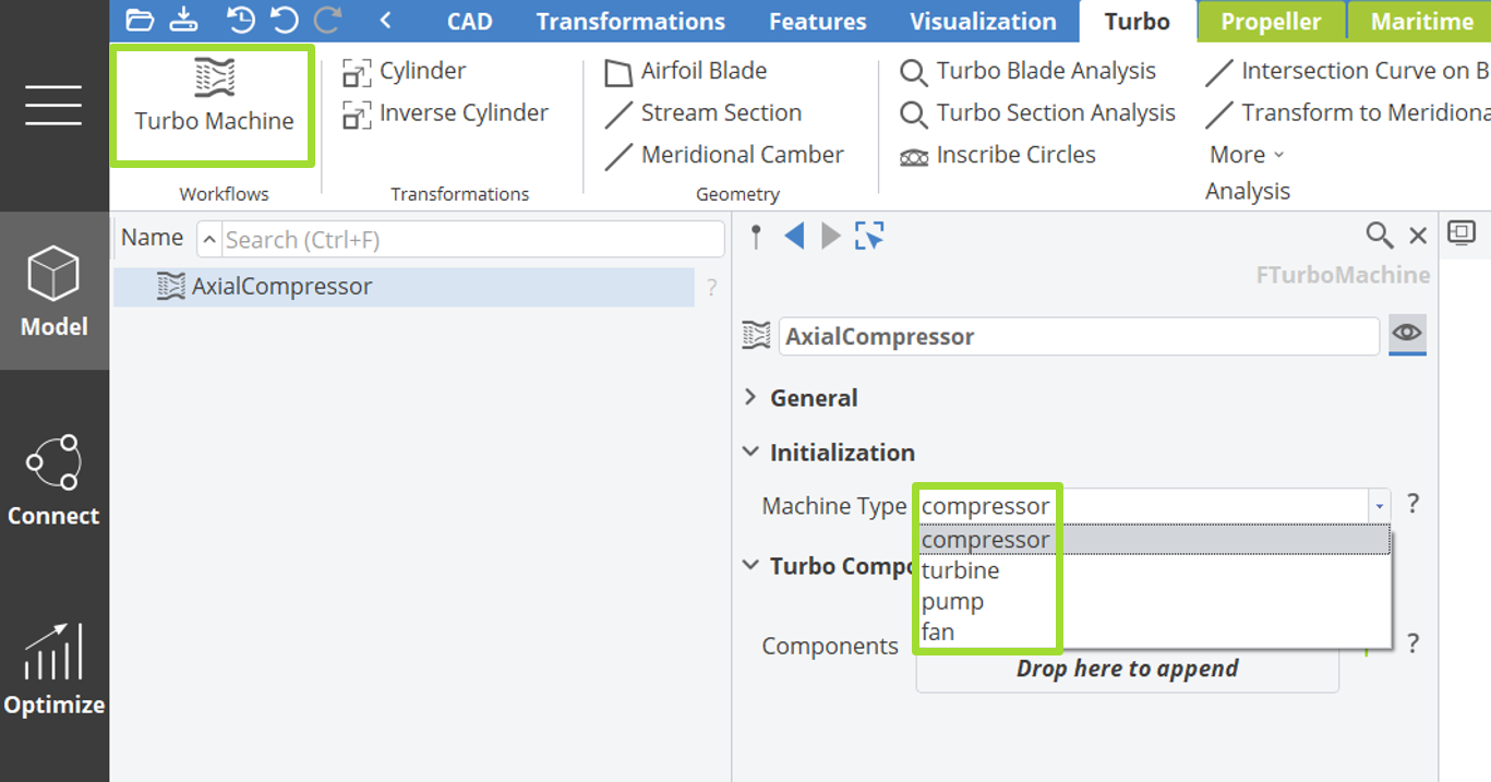Machine type selection

Step 2 | Component

It is now possible to add a bladed or unbladed component beneath the Machine Type selection. An axial bladed component could be a rotor or stator while an unbladed component might be a diffuser/nozzle shaped intake or some other form of flow guiding component. A bladed component is described by the meridional contours as well as the blade object.

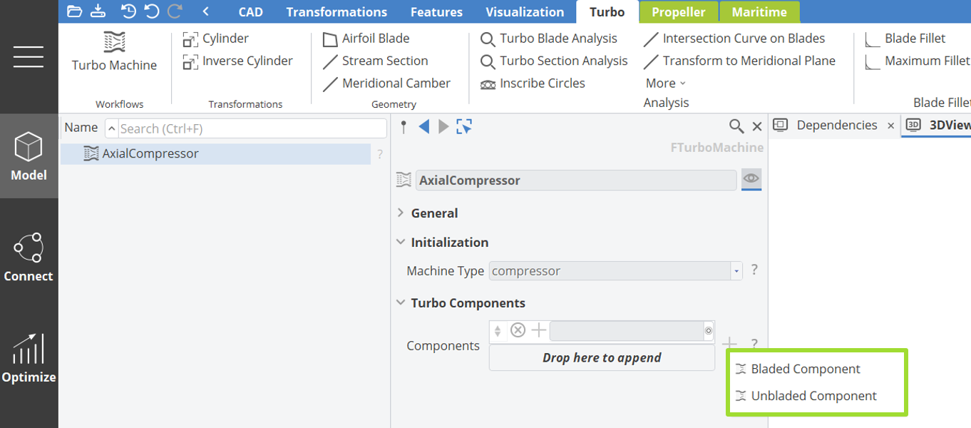Add a bladed component

Click on the green plus symbol next to the window Machine Type to reveal a drop down menu which includes the options bladed component and unbladed component. After a component is selected, a new object is generated automatically inside the object tree. Inside the bladed component object it is now possible to define the component's properties. By specifying the stage properties, CAESES will automatically suggest suitable features for a certain machine type. These properties include:

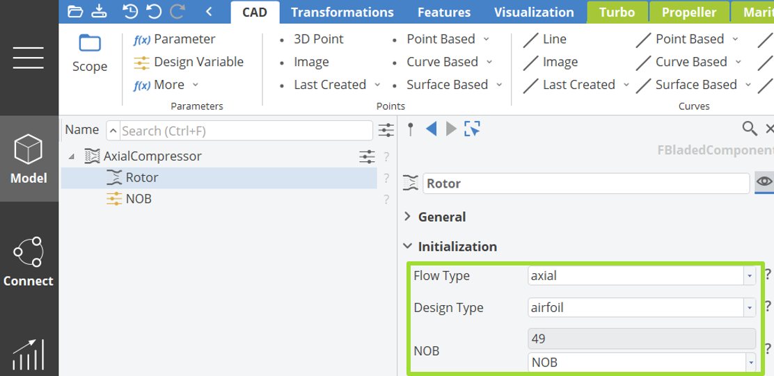Rotor definition with axial airfoil setting

Flow Type

The flow type determines whether the bladed component is a centrifugal/radial or axial flow machine. In this case, let's choose an axial flow based component.

The flow type will be used to initialize components like the FMeridionalContours object in the design workflow and will automatically suggest designated curve types or feature definitions.

note

If you want to design mixed flow machines you need to decide if the machine is more "centrifugal / radial" or "axial" and then adjust the suggested parametrizations to your needs, accordingly.

Design Type

With the design type the user can decide if the blade should be modeled based on a mean camber surface or directly with airfoils / hydrofoils. Axial turbomachine blades are using specifically developed airfoil definitions to minimize aerodynamic losses, which is why this approach is preferred when modeling an axial turbomachine component.

With the airfoil approach the user will model the blade profile definition in the 2D x,y - plane with a feature definition. Based on this definition the blade is created with the FAirfoilBlade, which will transform the 2D profile into 3D space based on a variety of transformations the user can choose from.

Number of Blades

Set the number of blades for your turbomachine or create a design variable for it, to easily change it.

Step 3 | Meridional Contours

Hub & Shroud Contour

After setting the fundamental parameters of the machine, the meridional contours are defined. For that, click on the plus on the right next to Meridional Contours, which will automatically generate the meridional contour object in the object tree. Here, it is possible to create contours with suitable curve types and parameterizations.

Let's start by creating the rotor's hub contour inside the meridional contour object by clicking the plus icon on the right next to the input field Hub Contour. When clicking the plus symbol, the workflow proposes two curve types inside a drop down menu (4 point tangent curve and straight line) which are often used when designing axial meridional contours. These options are only a general suggestion, which can be of course individualized by creating contours with user specific curve types. To insert custom curve types, you can simply insert your custom curve into the input field.

info

Note that when creating and inserting your custom curves inside the meridional contour object, the orientation of the curves needs to follow along the positive Z-Axis direction and the curves need to be defined inside the Y - (Z,X) -plane. Conventionally the curve orientations are the identical to the fluid flow direction in the Turbomachine Workflow or in CAESES in general.

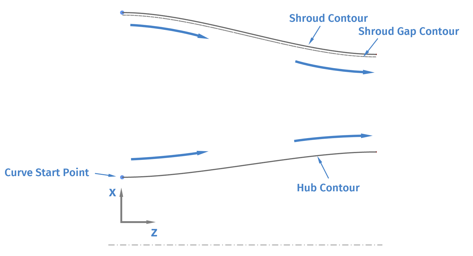Hub and shroud curve definition in the Turbo Machine Workflow

When choosing one of the proposed curve types, a new scope is automatically created in the object tree, containing all necessary objects. Change the values of the design variables to fit the desired dimensions by clicking the edit button next to each design variable. To show and edit parameters, select the parameter icon.

To create the shroud and shroud gap contour, simply repeat the steps from the creation of the hub contour. The shroud gap contour is created by a constant offset curve from the shroud contour. It is possible to define a linear distance distribution, by either changing the parameters offset1 and offset2. This can be individualized even further by inserting user specific curve types inside the Thickness Distribution input field found in the gap distribution curve.

tip

If you want to define a user specific distribution function e.g. for the shroud gap contour, the distribution curve needs to be defined in the Z - (X,Y) -plane and run from 0 to 1 along the X-Axis. This is due to the curve parameter t in CAESES, which runs from 0 to 1.

caution

The stacking axis must always run from hub to shroud for the Turbo Machine Workflow. If the orientation of curves is backwards, errors in the blade creation may occur.

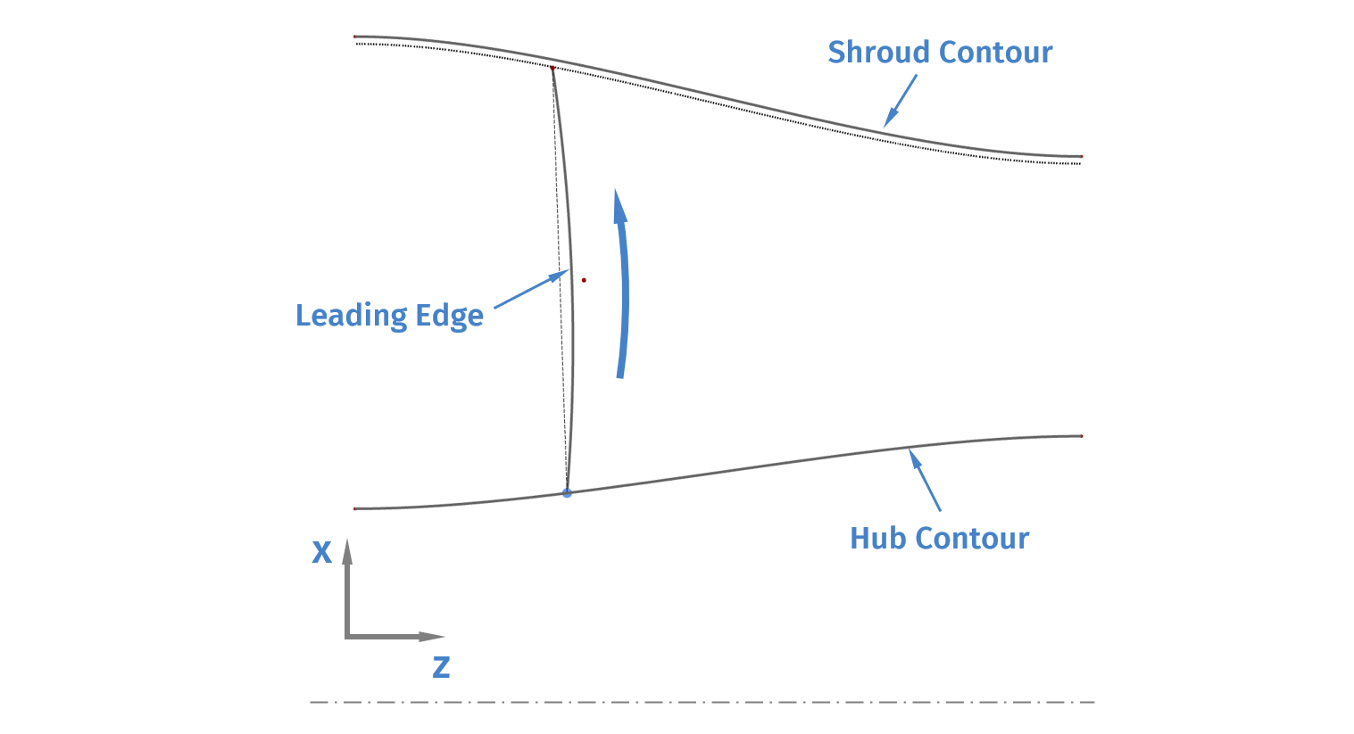Leading Edge Definition

Stacking Axis

Now let's create a radial stacking axis along which the airfoils is being stacked. To add a stacking axis, navigate back to the meridional contour object and click on the plus symbol next to the input field Leading Edge to reveal a drop down menu with several curve options. Since the airfoil blade feature creates the blade surface through a meta surface, complex stacking axis shapes can be realized while still generating a robust and topologically clean surface. To customize the stacking axis, simply shift the intermediate points towards the desired location by drag and drop or by specifying the point or curve parameters.

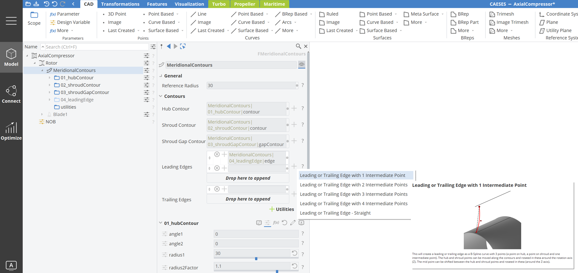
Stacking axis definition

To change the location of the start- and end point of the stacking axis along the Z-Axis, adjust the design variables posHub and posShroud. To also change the location of intermediate points along the Z-Axis, simply add a translation operation inside the section Operations in the Object Editor. The shift of the stacking axis along axial direction is called forward and backward sweep, depending on along which direction the blade is shifted. This is often used in transonic blades where backward sweep is used to tilt the shock on the suction side of the blade to reduce aerodynamic losses or forward sweep is used to minimize the formation of vortices at the leading edge e.g. the horseshoe vortex/stagnation vortex at leading edge. [5], [6]

For changing the location of the stacking axis in circumferential direction, alter the design variables thetaShroud and thetaInt. This shift is known as negative/positive lean or bow. Lean defines a linear shift along theta and bow as the name suggests is a circumferential shift with a non-linear shift, which can resemble the shape of a bow. The circumferential shift has an impact on the passage vortex and thus is used to also minimize aerodynamic losses by smartly affecting the complex interaction between the different vortex systems.

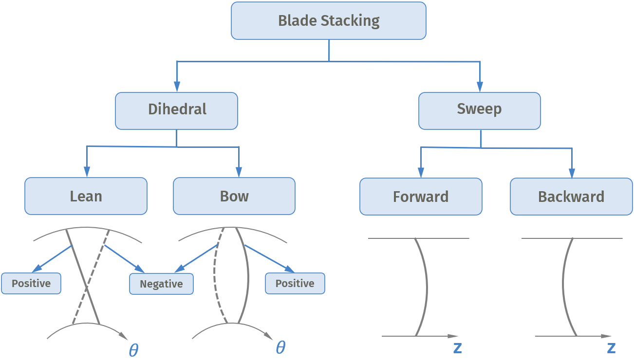Axial blade stacking methods

Step 4 | Blade Design

Now that the meridional contours are defined, the blade surface can be modeled. Navigate back to the bladed component object and click green plus next to Blades, which automatically creates the Blade object in the object tree. To create the blade's surface, simply click on the green plus symbol next to the input field Surface under the section Blade Surface. Since axial turbomachinery blades are commonly modeled with the airfoil blade approach, the drop down menu automatically suggests the Airfoil Blade object.

Create the axial blade surface

Airfoil Blade

The object type FAirfoilBlade lets you create a fully-parametric blade based on an airfoil profile definition in a matter of minutes. It combines a 2D profile (feature) definition – either user-coded, or from a list of templates – with a 3D transformation to directly loft a surface in spanwise direction from hub to shroud.

Choose between

• a cylinder transformation, which transforms the 2D profile onto a cylindrical surface,
• ZRT (z-r-$\theta$), which allows a transformation of a 2D profile onto a stream surface located between hub and shroud, where the x-coordinate corresponds to the z-position and the y-coordinate corresponds to the $radius\cdot\theta$ value,
• MRT (m-r-$\theta$) offers a transformation of a 2D profile onto a stream surface between hub and shroud, where the x-coordinate corresponds to the meridional m-position (streamwise arc length) and the y-coordinate corresponds to the $radius\cdot\theta$ value.

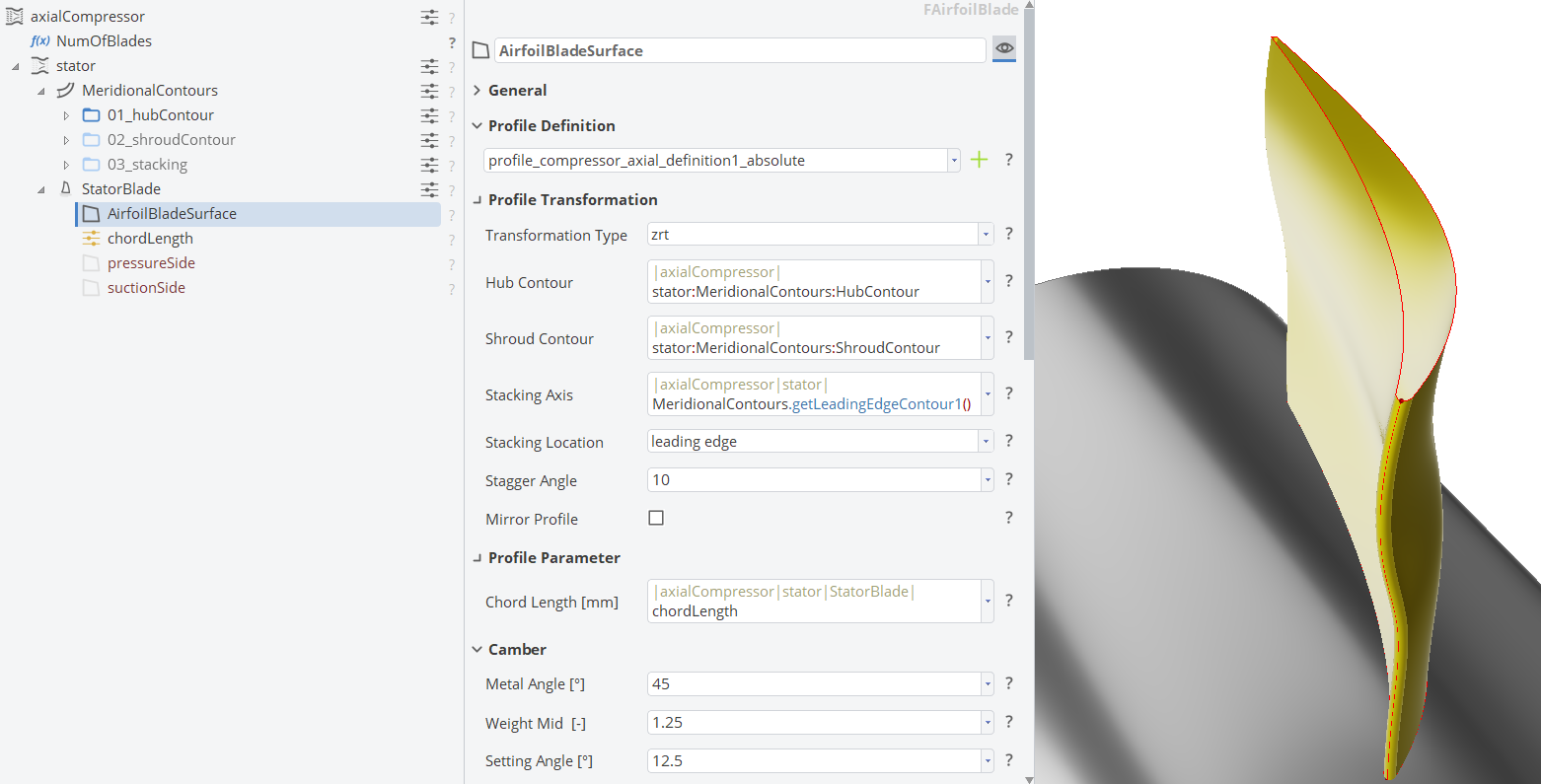
2D Airfoils

In order to achieve the redirection of the absolute velocity component, machine specific airfoils have been developed, which differ in shape and size depending on which purpose the airfoils have and in which environment they are applied. To select the blade's profile, click the green plus symbol next to Profile Definition inside the Airfoil Blade object to reveal a drop down menu with pre-defined compressor and turbine profile definitions. Each profile is available in absolute and relative parameters regarding the profile's thickness. For axial machines, CAESES provides three different types of compressor profiles and one turbine profile.

Compressor Airfoils

The first compressor profile definition is visualized in the following image (i) and is defined via the input parameters Metal Angle $\varphi$, previously defined as blade angle $\beta_{b1}$, the Setting Angle, also defined as stagger angle $\gamma$ previously, and Weight Mid, defining the distance of the middle point of the camberline NURBS curve. Since sharp profile edges are not feasible in reality, elliptic edges have been implemented, which can be customized by the ellipse radius and ellipse factor. The ellipse factor describes the ratio between the two ellipse radii and stretches or flattens the elliptical shape.

A second pre-defined compressor profile definition is based on the incidence angle $i$, the turning angle, also known as the deflection angle. Here, the elliptic shape of the leading and trailing edge can also be customized. This profile is shown in the next image (ii).

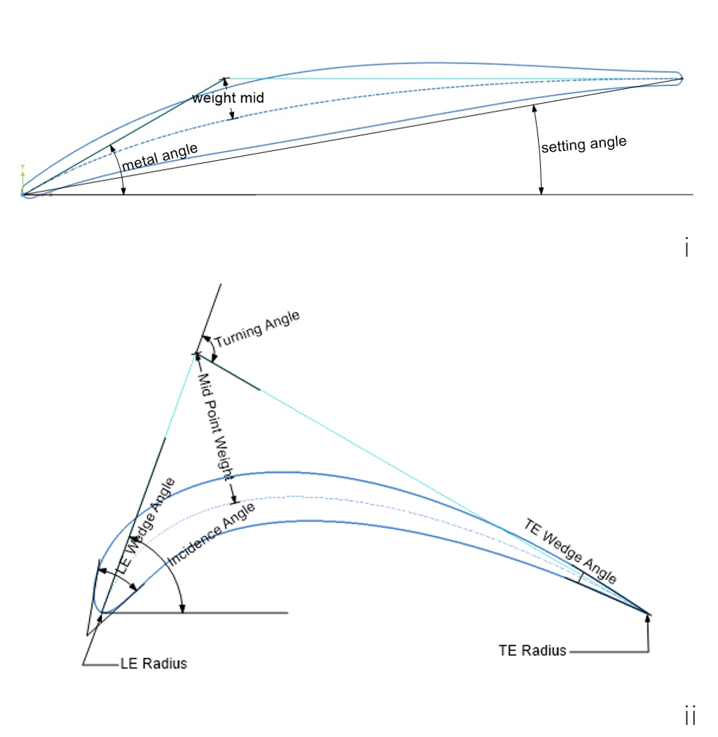i: Axial compressor profile via metal angle, setting angle and weight mid

ii: Axial compressor profile via incidence angle, turning angle and weight mid

The third profile option for axial compressors is the well known NACA-4-digit airfoil definition with an elliptical leading and trailing edge, shown in the figure below.

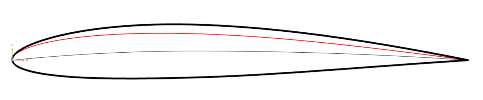NACA 4 digit profile

Axial Compressor Profile Families

NACA-6-digit Family

The often applied and most known profile family in axial compressors is the NACA-65-series, which is part of the NACA-6-digit family. These profiles were developed to shift the position of minimum pressure on the suction side downstream and smooth out the suction tip of the airfoil, resulting in low positive pressure gradients, which at the end leads to minimal aerodynamic losses and thus maximum efficiency. NACA-65 airfoils are used in subsonic and intermediate-transonic Mach numbers, $M=0.1-0.6$ [8].

C-Family

Another known subsonic profile family is the so-called C-family, where the C4-profile is a popular airfoil. Modern numerical methods lead to the development of Controlled Diffusion Airfoils (CDA), which are shape optimized airfoils resulting in a steady and controlled diffusion on the suction side. [2]

For transonic and subsonic axial compressor blades, Double Circular Arc (DCA), and Multiple Circular Arc, short MCA profiles, are used due to the sharp leading edge. On the other hand, sharp leading edges lead to a small operating window in which these profiles can perform.

Turbine Profiles

In contrast to compressors profiles, which are in constant threat of boundary layer separation, turbine profiles are not limited by a positive pressure gradient and thus don't need complex profile definitions, which need to fulfill blade loading criteria. But, due to the hot environment in which these blades need to operate, internal cooling structures might lead to relatively thick profile definitions. The Turbo Machine Workflow provides one pre-defined turbine airfoil definition, shown in the following image. This profile is defined through two angles, the metal angle, being the blade angle $\beta_{b}$, and the wedge angle, which defines the tangential angle between suction and pressure side, as well as the radius and the ellipse factor for the leading and trailing edge each. The two parameters suction side shift and pressure side shift define a perpendicular shift from the camberline of the profile, which results in the thickness of the profile.

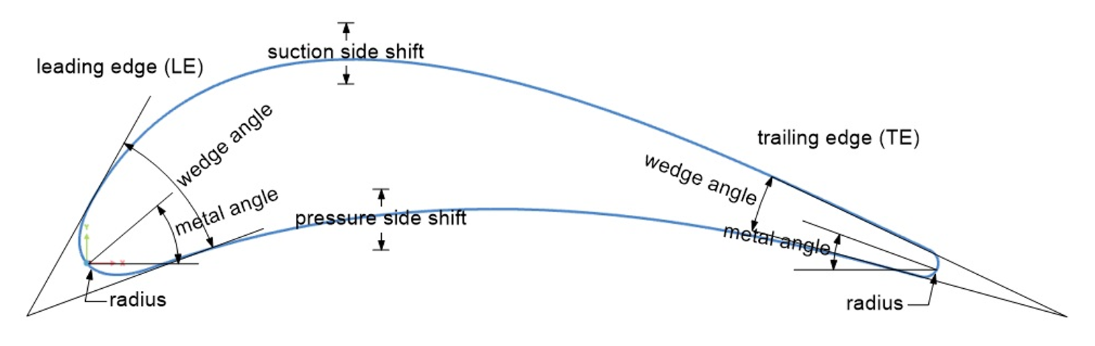Axial turbine profile

tip

When defining your own custom profile definition, the profile needs to be defined in the Z - (X,Y) plane and the chord length needs to run from 0 to 1 along the X-Axis. Also, if you would like to insert the custom profile definition into the Airfoil Blade feature, the profile must be defined inside a feature definition with the 2-dimensional profile curve as output, since the input type of the profile definition is FFeatureDefinition.

Step 5 | 3D Blade

The 3-dimensional blade is created through a meta surface by the Airfoil Blade object. This means, that the 2-dimensional profile curve is mapped into 3D-space by a specified transformation along the stacking axis. Meta Surfaces are defined by Curve Engines, where each input value can be described with a distribution curve, which then defines the change of the parameter along the mapped surface's V-direction. In this case, if a distribution curve is inserted into an input field inside the Airfoil Blade object, e.g. the blade's chord length, the parameter changes according to the distribution curve along the blade height.

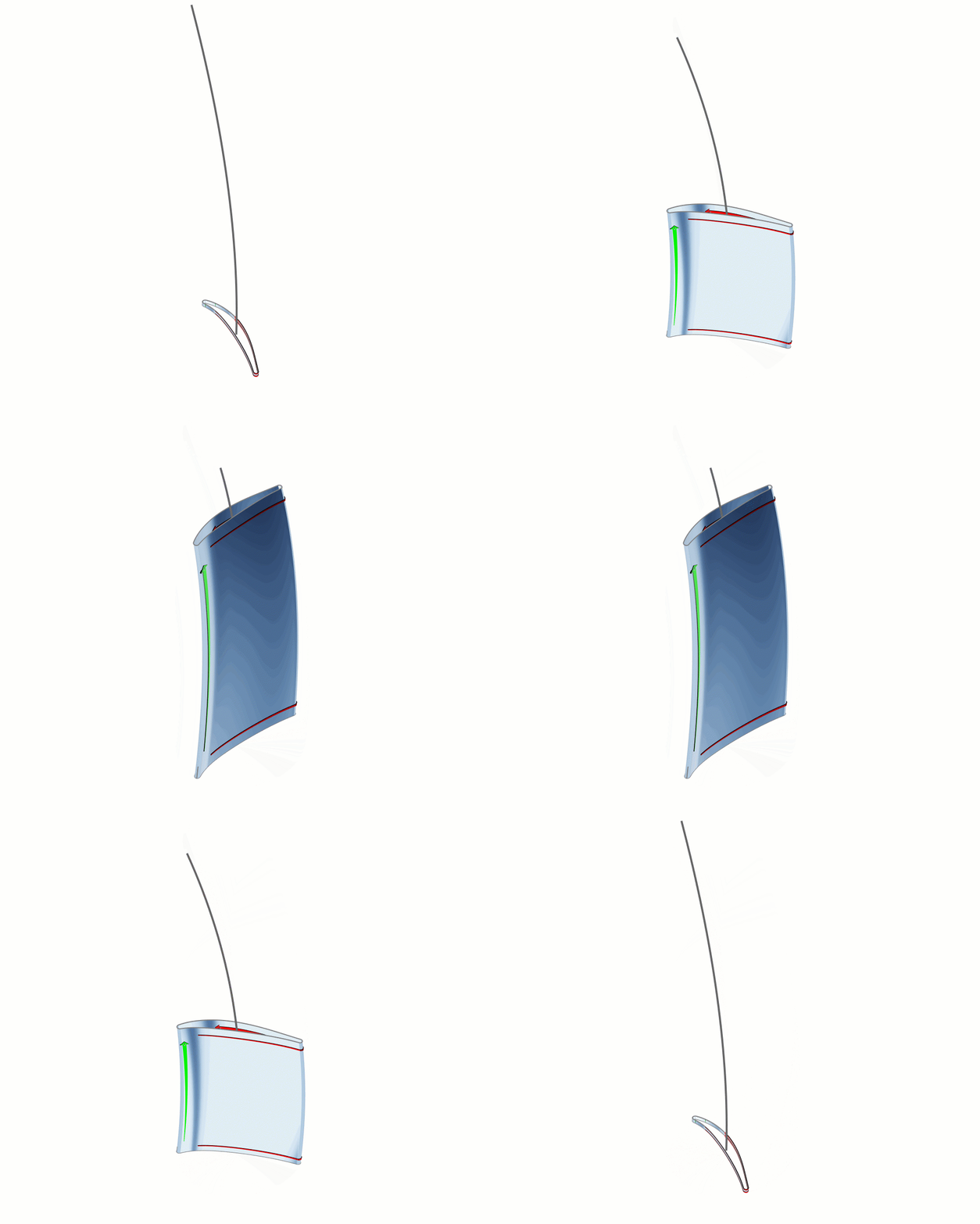
Transformations

The Airfoil Blade object offers four different types of transformations:

1. zrt ( = z-r-$\theta$): This transformation maps the 2D profile section into the z-r-$\theta$-space. Here, z is the main axis in axial direction, r is the radius of the machine and $\theta$ relates to the rotation around the Z-Axis in the Z - (Y,X)-plane.
2. mrt ( = m-r-$\theta$): Here, m is the meridional streamline, which creates 3-dimensional shape as shown in the general structure overview.
3. cylinder: This transformation transforms the 2D profile onto a cylindrical surface.

After the airfoil blade object was created in the object tree, the profile is automatically referenced and the 3D-transformation can be selected from the drop down menu next to Transformation Type under the section Profile Transformation. The hub and shroud contour as well as the stacking axis are referenced automatically. Since the airfoil blade is created through a curve engine, it is possible to insert distribution curves for each profile or blade parameter.

Blade Distribution Functions

To create blade distribution definitions from hub to shroud, curves can be created in the Z - (X,Y)-plane, which run between 0 and 1 along the X-Axis. There is no limitation on what type of curve can be used for a distribution function. A common practice is to use B-Spline or Interpolation Curves. Another type of curve that is often used for distribution functions is the Planar Curve with Tangent Control to determine a certain gradient at the start and end of the curve. For a better overview, blade distribution curves are defined with a normalized Y-value for the given parameter. The value of the parameter can be scaled to the correct value later on inside the input field of the airfoil blade object.

The airfoil blade object also offers the possibility to create pre-defined distribution curves by clicking the green plus symbol on the right next to each blade parameter. When clicking on the plus, a drop down menu offers three different type of distribution curves, being B-Spline, Tangent Control and Interpolation. Blade functions can be parameterized by e.g. creating parameters that describe the positions of the control points or other parameters that are used to define the curve. Mostly, this part of the design process is the most complex as it can be challenging for engineers to find the optimal parameterization of the geometry and thus find the balance between the minimum amount of degrees of freedom of the parameters, which is important to scale down computation resources, while still being able to reach a maximum of shape variation, which defines the potential of the shape optimization. A smart parameterization is essential for an efficient optimization.

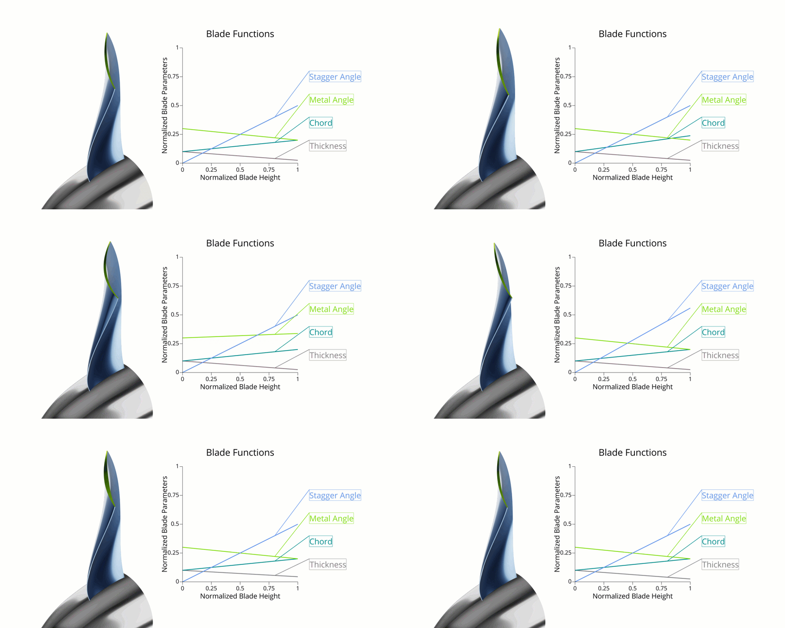
The parameterized distribution functions can now be inserted into any input field inside the airfoil blade object or if they were created by the green plus symbol, they should be referenced automatically. After referencing the distribution functions, a number emerges next to the distribution curve, which is per default 1. This parameter is the scale factor of the distribution function, which scales the normalized values from the function towards the original values. It is also possible to insert a negative scaling factor, which will then lead e.g. negative stagger angles.

Stacking Axis

In the airfoil blade object, it is possible to choose between two different methods of stacking:

1. Leading Edge: Stacks the blade profiles at the leading edge.
2. Center of Area: Stacking line lays at the center of area (COA) of each airfoil section.

Additionally, if the blade needs to be cambered into the opposite direction, toggle the button Mirror in the Profile Parameter section.

Axial Turbomachinery Samples

Take a look at the sample models for

• an axial fan,
• and an axial compressor stator with endwall contouring.