Hull Variation with Delta Shift
In this tutorial you will learn how to vary existing hull geometries using the Delta Shift transformation. For demonstration purposes, an IGES file is imported and the hull shape gets varied i.e. “shifted”. This kind of partial parametric modeling technique can not only be applied to imported geometries such as IGES, STEP or STL files, but to any geometry models existent in CAESES. In addition, Delta Shift transformations can also be applied to offset data (e.g. used by the CFD package SHIPFLOW).
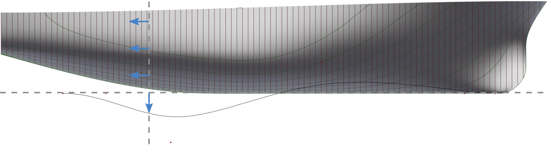
In hull design, the Delta Shift is typically used to shift initial geometry in x-direction according to a given shift function. In the present case, the abscissa of the shift function is the x-axis while the ordinate is the z-axis. Geometry information at a specific x-position (you can think of an individual section at a position x0), is then shifted with the corresponding z-value of the function at x0. Negative z-values move the shape at x0 backwards while positive values represent a forward shift.
By keeping the applied shift function continuous with smooth (horizontal tangent) start and end, the resulting hull shape will stay fair while the technique allows to easily change hydrostatic characteristics of the vessel to a great extent.
Applying a Delta Shift to a hull in this manner allows to directly and distinctly change a hulls Sectional Area Curve.
Initial Geometry
As mentioned earlier, this tutorial will be based on an imported hull geometry. However, the subsequent steps may also be applied to any model generated within CAESES.
- Save the geometry file:
-
Choose (Hamburger) Menu > Import* Tab > IGES and select the
basicOSV.igsfile you saved -
Rename the newly generated Scope to “geometry”.
-
Rename the two surfaces to “main” and “stem” for easier differentiation.
-
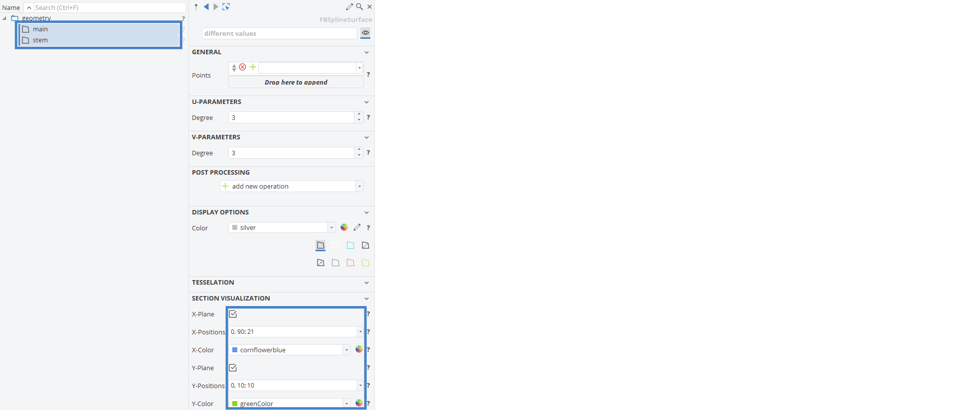
Select the two surfaces and visualize some sections in x-direction (i.e. expand Section Visualization in the object tree). Toggle to activate and set a series for each plane you want to visualize.
Shift Function
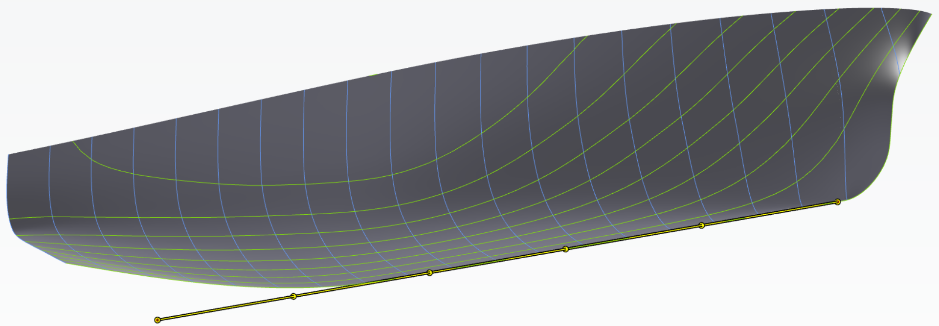
In this step we create a shift function. It will define the way the hull is shifted in longitudinal direction. To leave the stem surface and the stern area unchanged, the shift function will be defined in the range of x = 10m to x = 80 m.
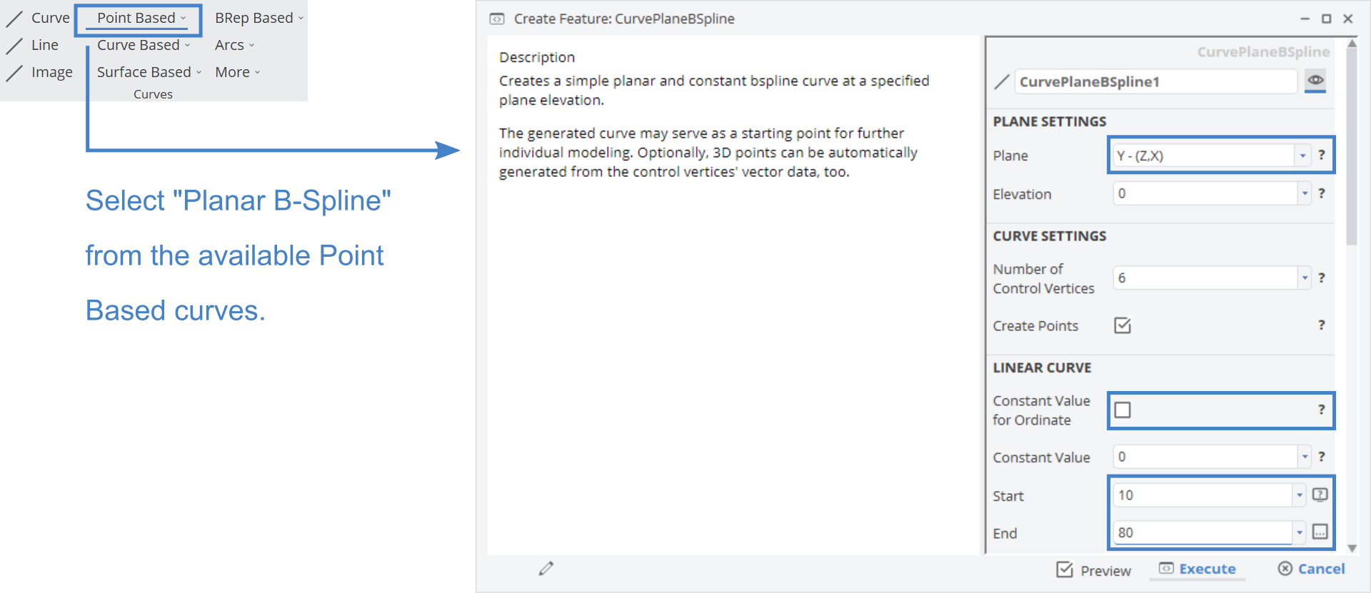
- From the available curves in the CAD tab of the Model workspace, create an initial planar B-Spline curve:
-
Set the Plane, as well as the values for Start and End, according to the screenshot above.
-
Deactivate Constant Value for Ordinate.
-
Press the Execute button.
-
Rename the newly created Scope to “shiftFunction”.
Delta Shift Transformation
CAESES offers a wide variety of partially-parametric modeling techniques out of which this tutorial will focus solely on the so-called Delta Shift transformation.
-
In the CAD tab of the Model workspace, within Transformations, choose Shifts > Delta Shift and name the new object “shift”.
-
Activate Delta X and insert the shift function from the previous step as a Deltacurve.
-
Activate x-abscissa and z-ordinate as shown in the following screen shot:
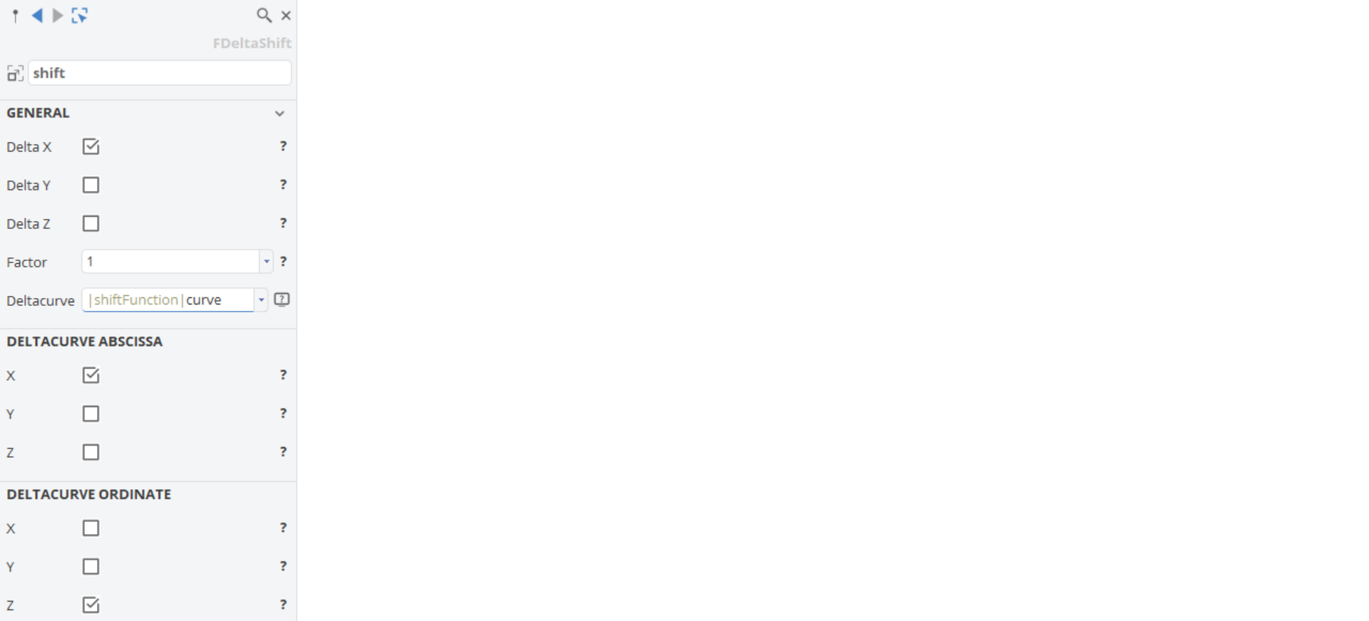
The attribute Factor scales the values of the shift function. This is useful if the shift function provides very small values for small changes of the hull and you still want to visualize the function in a scaled, larger version in the 3D view (you would set a Factor of e.g. 1/10).
Image Surface
An image of the initial surface is created which will receive the transformation.
Using an Image Surface is the method of choice whenever a surface should receive a transformation and a surface is also the type you wish to continue working with. Similarly, an Image Trimesh can be used when working with a Trimesh, an Image Section Group when working with Section Groups, etc. Note that BReps may receive transformations as a post-processing step.
-
Create an Image Surface by choosing Image from the Surface Based surfaces within Model > CAD.
-
Rename the newly generated surface to "newHull" and assign “main” as Source of “newHull”.
-
Choose the “shift” transformation as input for the attribute Image Transformation.

If you want to have the same section visualization for “newHull” as for main, copy visualization settings from one object to another by using the copy format from the context menu (right-click).
- The y-sections for the new hull are deactivated and the color of the x-sections is changed to "red" for a good comparison here.
Shape Variation of the Hull
The initial and the new surface are currently identical since the shift function has a constant value of 0.
-
Select p02 inside the scope shiftFunction|auxiliary and move it in z-direction (remember: this is the ordinate of our shift transformation).
-
Select p03 and move it e.g. in opposite z-direction.
-
Move p01 and p04 along the x-axis for more degrees of freedom. Keep the z-value for these two points at 0, in order to have a smooth transition to non-deformed geometry.
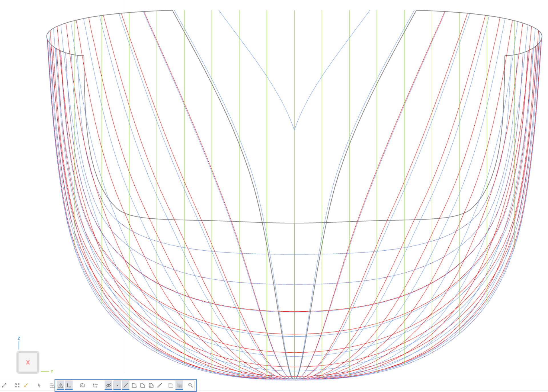
Use filters and mirroring options from the bottom of the 3D view to get a good look at how the two different hull shapes compare to each other. You can see how the modified hull shape is much more slender both, in the aft- as well as fore-body.
Conclusion
In this tutorial a Delta Shift transformation is applied to an existing hull. The shift is defined by means of an arbitrary user-defined curve. Instead of just dragging points manually, the x- and z-coordinates of the shift function could be controlled by design variables: a Design Engine could then automatically apply changes to the hull with regard to the chosen variation or optimization strategy.
There are other shift transformations available such as the Surface Delta Shift. Here, a surface is defined which provides the delta values for a certain principal direction. Both Delta Shifts and Surface Delta Shifts are frequently used in hull design to modify hydrostatic characteristics of an existing vessel. To do so in a more sophisticated way, the generalized Lackenby is an extended version of the presented Delta Shift where delta functions are internally generated. The resulting functions are created in a manner in which certain user-defined constraints are fulfilled, for instance a distinct percental change of the center of buoyancy or displacement.
CAESES Project File
If you want to take a look at the finalized parametric model you can find the resulting CAESES project file hull-variation-delta-shift.cdb here: