Generalized Lackenby Transformation
In this tutorial you will learn how to apply a Generalized Lackenby Shift to an existing geometry. A troubleshooting section is included at the end of this tutorial.
A Lackenby transformation is a method used in naval architecture to modify the hull form of a ship systematically by adjusting its sectional area curve. This transformation shifts volumetric distribution longitudinally, enabling designers to fine-tune parameters for improved hydrodynamic performance.
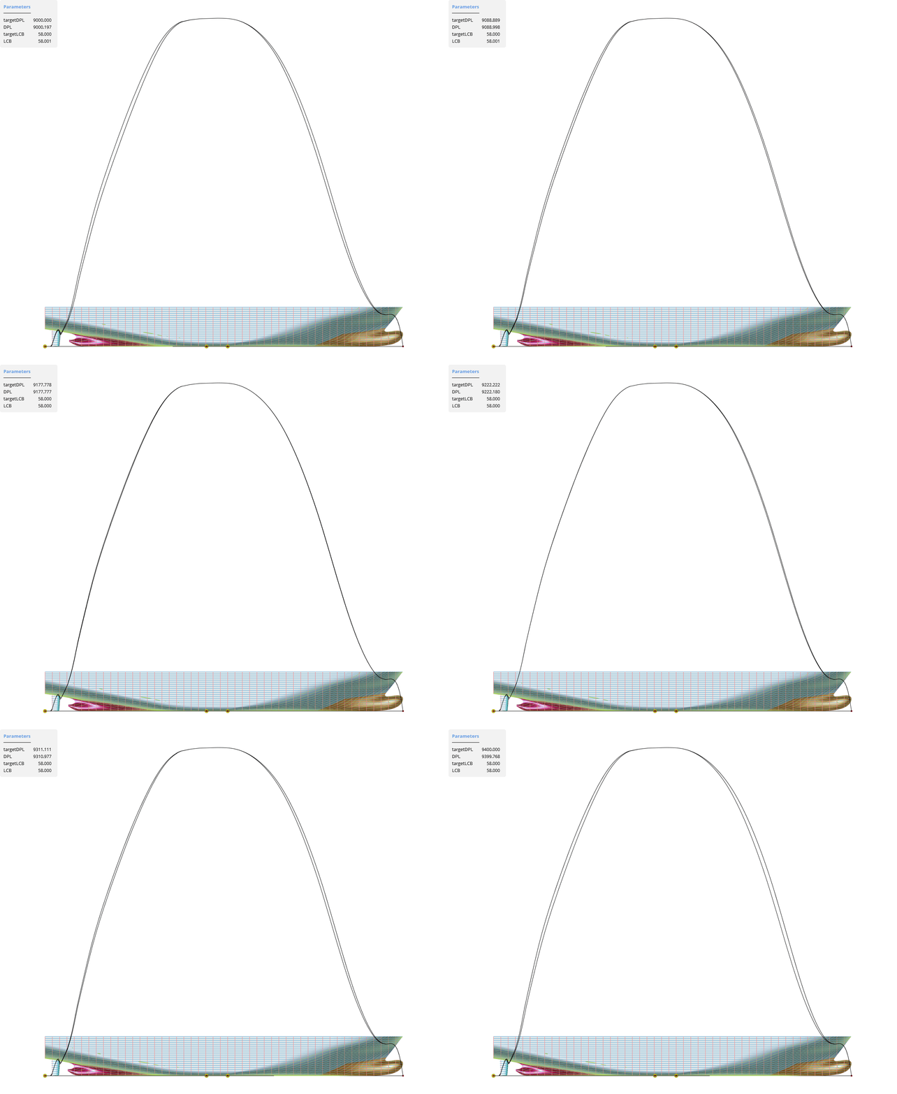
Variation of the displacement:
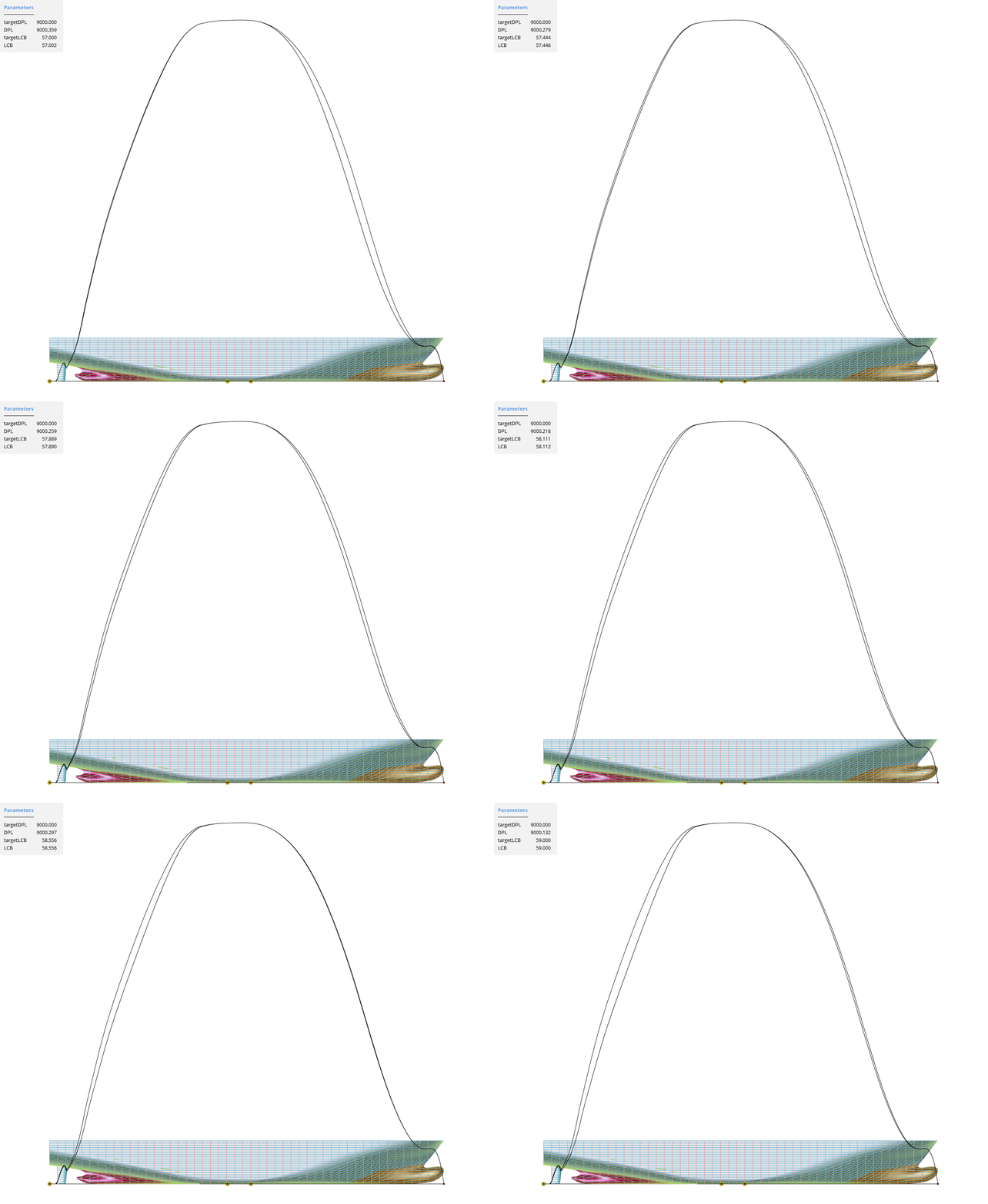
Variation of LCB:
In addition, the position and length of the parallel mid ship can also be modified.
For more information about the concept of shift functions you can also take a look at the Hull Variation with Delta Shift Tutorial.
Background
Let us start by exploring the significance and value of this concept in ship design and optimization. Incorporating a Generalized Lackenby transformation into a model ensures that all designs precisely meet the designer's requirements with respect to displacement (alternatively block coefficient or prismatic coefficient) longitudinal center of buoyancy, mid-ship position and length of the parallel mid-body. Rather than comparing various shapes, monitoring these values and posing constraints, each and every geometry will simultaneously fulfill all of these requirements and accurately match a specific target value or cover a distinct, given range. This eliminates the need for costly nested optimization routines or even manual fine-tuning. By running CFD simulations for the exact targeted displacement, the optimization can be expected to converge much faster and thereby lead to a superior results more efficiently.

There is a separate Lackenby Transformation in Model > Transformations tab. However, in this tutorial we will follow a simpler approach in which the Sectional Area Curve and Implicit Hydrostatics functionality are leveraged. These are easy to use, robust and flexible workflows available to users with the required license package (Maritime Add-on).
Import
Start by saving the STEP file we will use as a starting point and import it into CAESES.
Download Hull STEP FileRename the imported hull to "hull" and place it under the |00_import scope.
Sectional Area Curve (SAC)
The Sectional Area Curve (SAC) is a graphical representation of the cross-sectional areas of a ship's hull plotted against its longitudinal position along the length of the vessel. It is a fundamental tool in naval architecture used to describe the volumetric distribution of the hull.
- Create a new scope "01_sectionalAreaCurve"
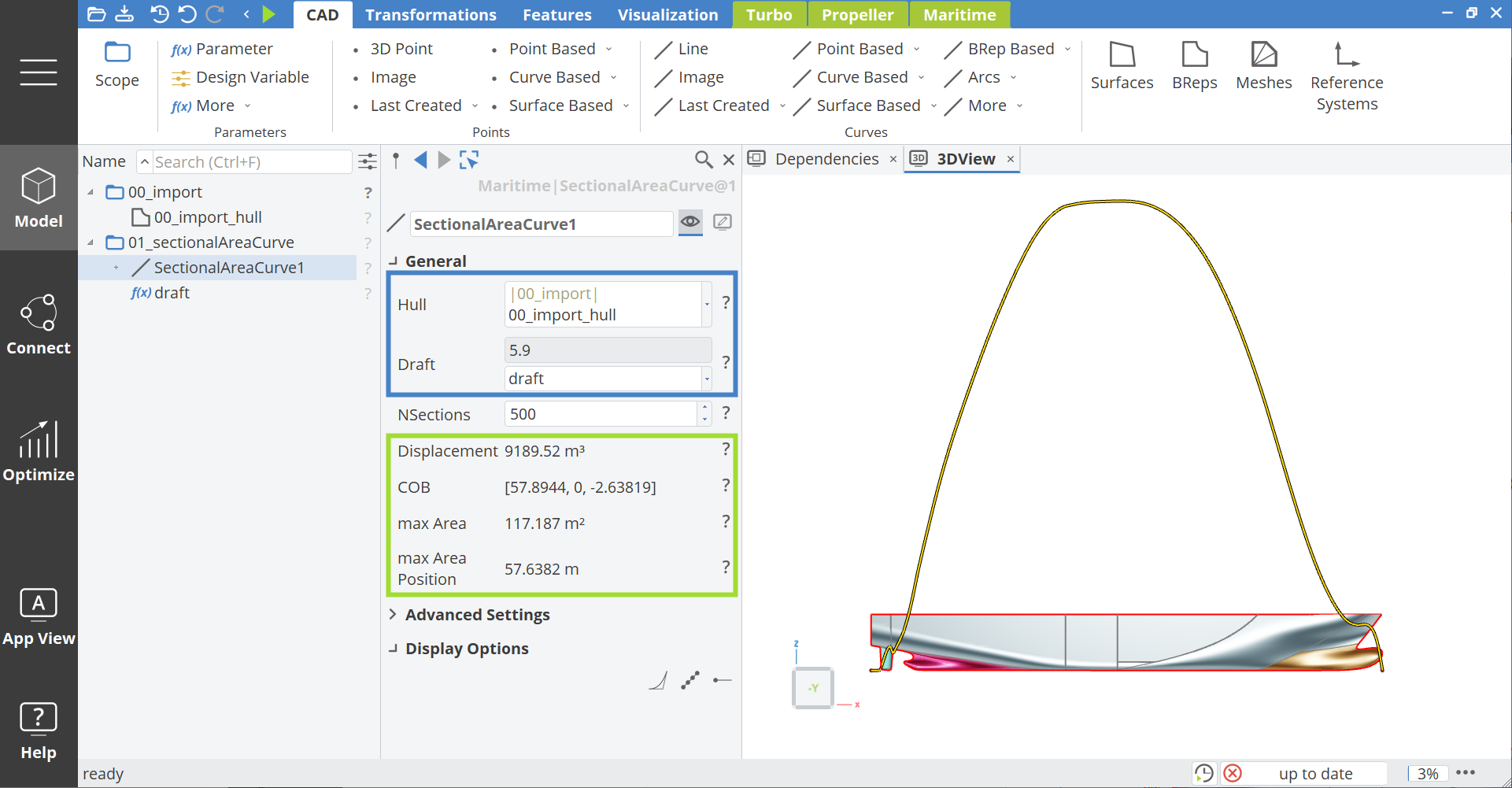
- Inside the scope create a Sectional Area Curve via Model > Maritime > Monitoring > Sectional Area Curve.
- Choose the imported hull and create a parameter named "draft".
- Set the value of the draft parameter to
5.9m.
Generalized Lackenby Transformation
The Generalized Lackenby method involves determining Delta Shift functions that inherently satisfy specific constraints. These constraints include changes in displacement and center of buoyancy, as well as precise start and end positions, tangent settings for the internal delta curves, and the placement of the mid frame. In this tutorial, we will bypass the complexities of setting up this process and instead utilize a pre-configured method conveniently available in CAESES.
- Choose Via Lackenby from Model > Maritime > Pre-Processing > Implicit Hydrostatics.
This will create a Transformation that requires a SAC as an input argument. With no additional parameters configured, the Object Editor looks as shown in the following screen shot.
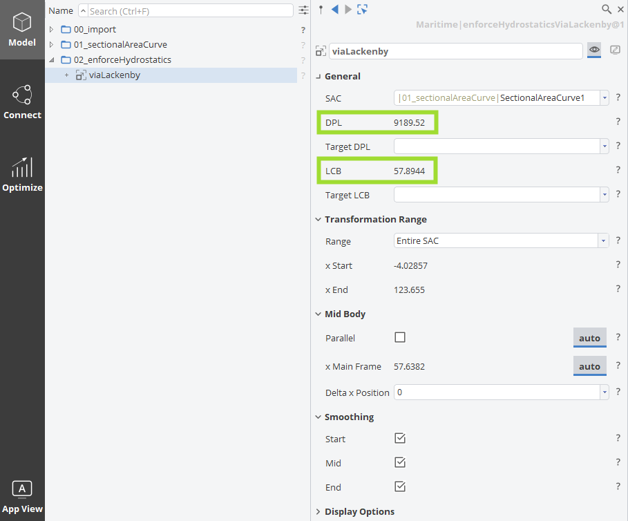
The current displacement volume (DPL) and Longitudinal Center of Buoyancy (LCB) are shown in the editor right away.
At this stage, we will define a target displacement and longitudinal center of buoyancy (LCB) before applying the transformation to examine the resulting geometry. The detailed configuration and settings will be addressed subsequently.
- Specify a target displacement (Target DPL) of
9000m³ and a Target LCB of58m and create a parameter for each value.
Apply Transformation
- Create a new BRep from the imported hull by assigning it as a source abd name it "hullModified".
- In the Post Processing category, the previously configured Lackenby transformation can be assigned.
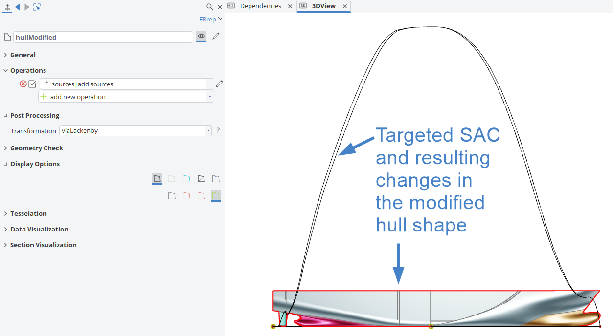
The modified hull will look very similar to the original one. Upon closer inspection of the original and target SAC, as well as the two BReps, deviations will be noticeable, depending on the chosen target values for LCB and DPL.
Verification and Accuracy
To double check that the transformation has had the desired effect on the hydrostatic characteristics of the hull, we will create another SAC from the modified hull BRep and choose the same draft as initially.
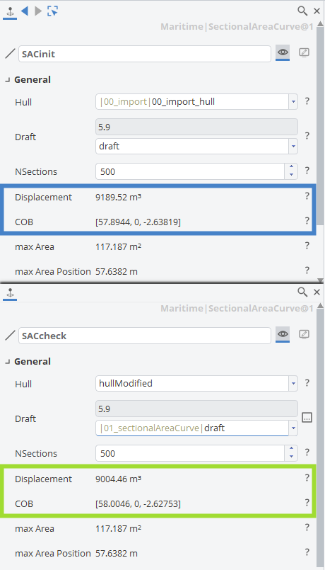
The results, in this case already show a very accurate match of 0.05% error in the displacement and 0.008% (less than 1 mm!) in LCB. Still, depending on the density of the control polygon of the initial hull and the tesselation settings (hydrostatics are calculated based on the triangulated geometry representation) the user might want to improve accuracy even further. If we set the Maximum Chord Height to 1e-5 for both the imported and modified hulls, and the Knot Spacing of the modified hull to 1, we obtain a near perfect match:
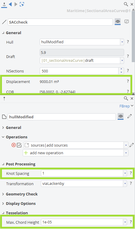
The resulting accuracy of far beyond reasonable practical requirements. However, it might be good practice to verify that the procedure works as intended and decrease the knot spacing and tesselation slightly from this point to ensure the project still updates quickly and is convenient to work with.
Keep in mind, that the Maximum Chord height setting must be specified for both, the imported and modified hull. For the knot spacing either one will do.
Detailed Settings
So far, we have only specified target measures for DPL and LCB. Users may specify the prismatic or block coefficient in place of displacement if preferred by calculating the corresponding values separately. However, there are a few more options to choose and set:
Transformation Range
Within the Transformation Range category of the method, the affected range can be specified. Any geometry outside these longitudinal bounds will remain unchanged and the transformation is limited purely to the given interval. For convenience, the entire length if the hull ("Entire SAC"), as well as the interval in which the submerged volume lies ("Submerged Volume") are extracted automatically and can be chosen. If non of these options fulfill the users requirements, a custom range may also be specified. This might be interesting if, for example the position of the boss cap or propeller shall remain unchanged.
Mid Body
In the Mid Body category, a Parallel midship option is available. If toggled, the parallel mid ship range can be specified (or auto-detected from the horizontal range of the SAC). The change in length, as well as the change in position can be specified and will be achieved along with the targeted DPL and LCB.
Smoothing
Finally, a Smoothing option is available for the start (aft), mid and end (fore) of the transformation. If all smoothing options are enabled, the resulting geometry will be changed gradually towards these x-positions. This is necessary in all cases, where the transformation is applied away from the overall extents of the hull or for hull shapes without a parallel mid ship section.
If set to false, the applied shift function will not start with a zero-tangent. As a consequence, the shift is not introduced gradually but rather abruptly in these positions. If a shift starts at the very aft of the hull, this does not affect the fairness of the resulting geometry. However, if it starts e.g. in the propeller plane, it is important to keep the transition from the unchanged towards the modified geometry smooth. The same holds true for the end position.
In the mid ship region, in cases of a parallel mid ship, it is not important to keep the shift functions smooth.The geometry itself has a "zero-tangent" in x-direction. Meaning it does not change in longitudinal direction as is the definition of a "parallel" mid ship.
If the transformation range includes the entire length of the ship, or if a parallel mid is present, choose false in these locations. As a result, the same change in hydrostatics can be obtained with a more homogeneous shift. In all other cases make sure to keep the function smooth in the respective areas. This is particularly important for geometries with high control polygon density (low knot spacing values) and across patch boundaries.
Troubleshooting
The transformation is, as is always the case with BRep transformations, applied to the underlying control polygon. Hence, a sufficiently high density of the control polygon is needed in order to keep the geometry watertight. If open edges show up in the modified hull, try increasing the number of control points by choosing a small Knot Spacing value (begin with approximately one percent of the ship length).
If the hydrostatic measurements are off by a little, try a finer Tesselation (i.e. 1e-5 vs. the default setting of 1e-4) for both, the original and modified geometry. In addition, choose a smaller knot spacing (begin with approximately one percent of the ship length).
If the transformation is slow, try to increase the Tesselation back to the default 1e-4 for both BReps. Check if the transformation still works robust and accurately with slightly larger Knot Spacing. If the increase in CPU time results from down-stream elements in the project, try a Data Reduction for the modified (and potentially also the initial) BRep. This will reduce the control polygon density while keeping the resulting shape changes within the specified tolerance (begin with e.g. 0.001 which corresponds to a maximum deviation of 1 mm for a ship modeled in m).
If the mid frame position and length change slightly different than they are supposed to, check the automatically determined start and end position of the parallel mid. Manually specify the exact values as per your requirements if necessary.
CAESES Project File
If you want to take a look at the finalized parametric model you can find the resulting CAESES project file lackenby-hull-variation.cdb here: