SHIPFLOW Connection
SHIPFLOW CFD Analysis
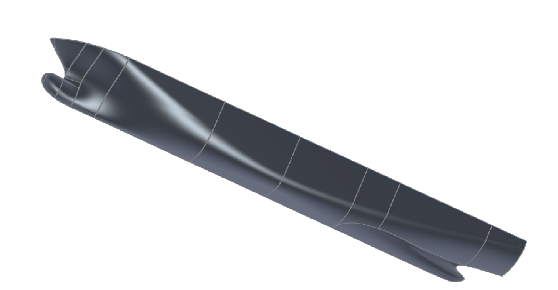
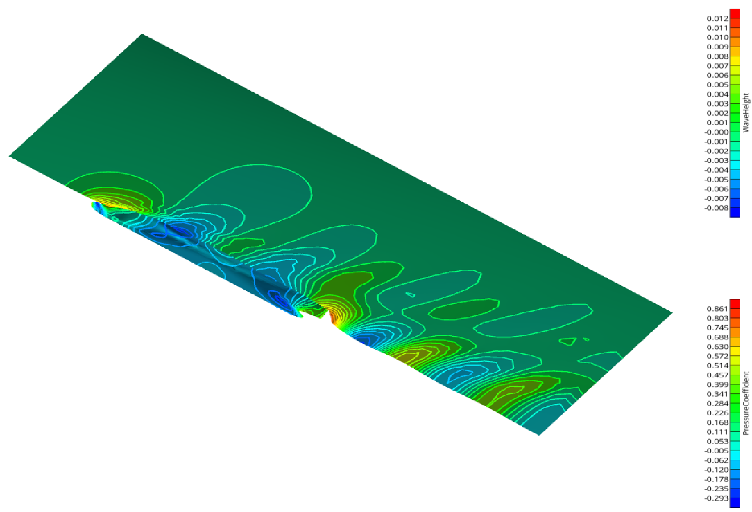
This introductory tutorial shows how to run the CFD-package SHIPFLOW from within CAESES. In order to keep it simple, an existing IGES geometry is utilized. The CFD settings are configured and a computation gets run finally. The calculation results can be accessed and post-processed, for instance, wave patterns can be visualized in the 3D view.
Initial Geometry
The hull needs to be imported first. Instead of using an existing IGES geometry, the subsequent steps do also apply for any parametric model that has been created in CAESES.
-
Download the IGES file of the container vessel we will use for this tutorial
Download IGES -
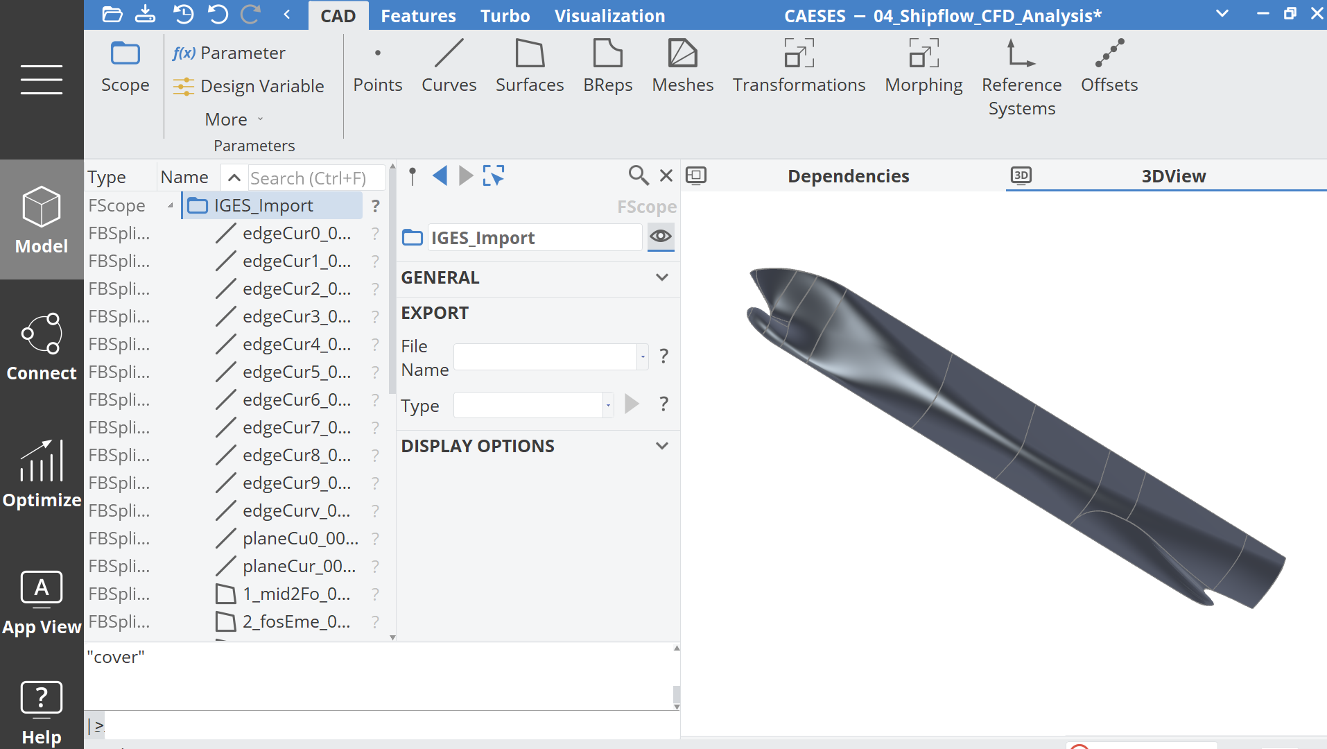
Go to Menu > Import > IGES and import the container vessel.
Surface Group
We need to assemble all surfaces in a surface group to have a single object for the upcoming SHIPFLOW configuration.
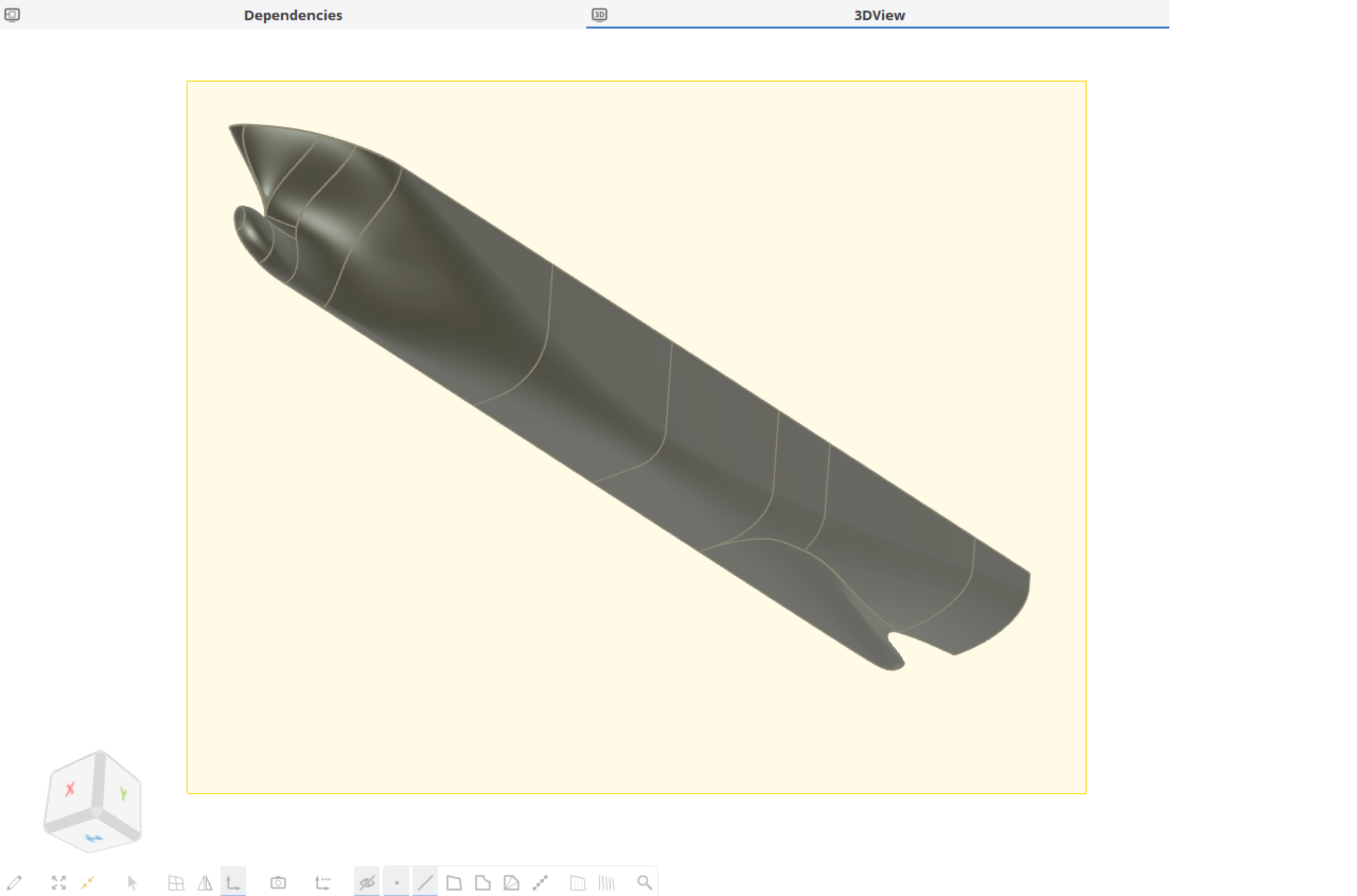
- Deselect all curves in the 3DView (1)

- Select all surfaces either in the 3D view or in the object tree.
-
While the surfaces are selected, choose Model > CAD > surfaces > surface based > surface group.
-
The initial default name of the created group is “grp1”. In order to have a more meaningful name, let’s name it “hull”.
Creation of SHIPFLOW Setup
CAESES provides convenient pre-defined setups for SHIPFLOW for quick and easy configuration:
- Choose Connect > SHIPFLOW* which creates a configuration and a computation in the tab connections.

Now, we need to set up the configuration of SHIPFLOW:
-
Expand the object “configurationShf1” in the tree and select xflow. (1)
-
Choose offset from the pull-down menu of the xflow entry and press the plus-icon next to the pull-down menu. (2)
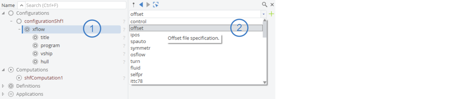
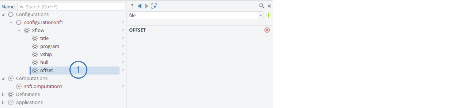
- Select the offset entry and, in the same manner, add iges, lpp, xaxdir, ysign, xori and zori.
SHIPFLOW Geometry
The created configuration and its entries can now be filled with project-related values and geometry:
-
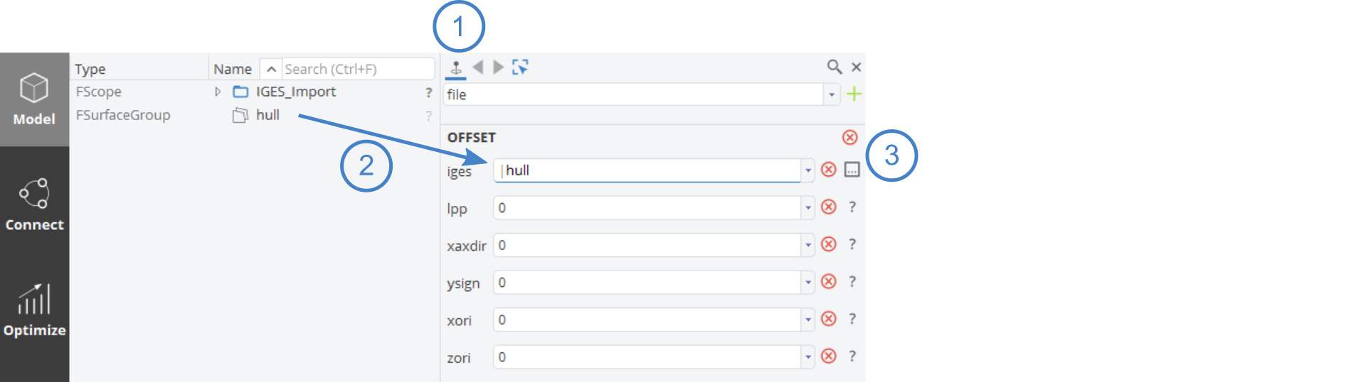
Click on the Model tab for access to the geometry (the offset entry is still pinned). (1)
-
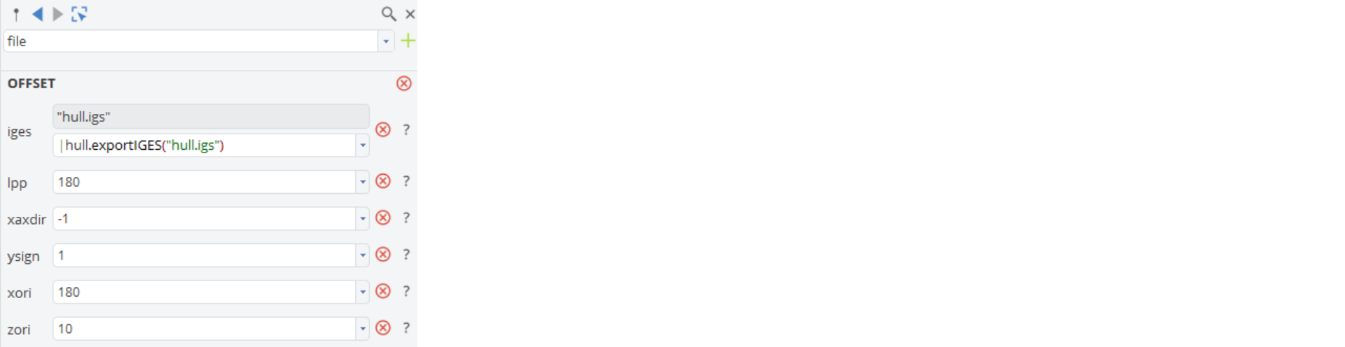
Drag and drop the surface group “hull” into the IGES field of the offset entry. (2)
-
Click at the auto-completion icon (“…”) next to the editor field. (3)
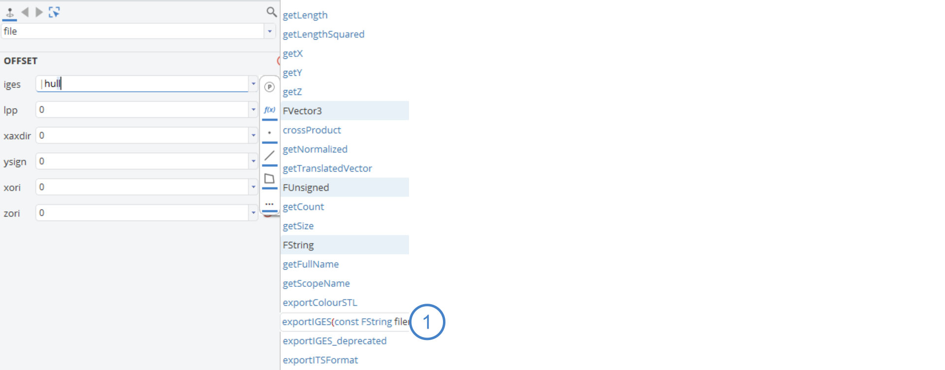
- Choose exportIGES(FString) from the list and set a name for the geometry file. This command will export all surfaces. (1)
- Enter the remaining values according to the screenshot. All additional settings are just defining the coordinate system for SHIPFLOW computations positioned at forward perpendicular backwards orientated.
SHIPFLOW Main Settings
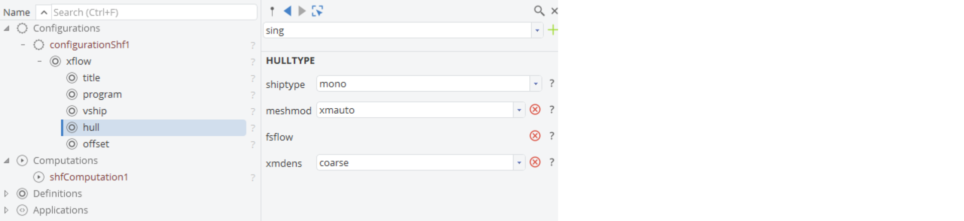
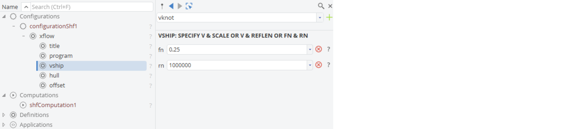
SHIPFLOW requires settings for defining the ship type (mono hull), an automatic mesh generation, a free water surface (fsflow) and a coarse mesh, due to computational time reduction. For other computations a coarse mesh might not be efficient enough. CFD speed calculations have to be set as well. Froude and Reynolds numbers are sufficient.
- Select the hull entry and add ship (“mono”), fsflow and xmdense (“coarse”):
- Select the vship entry and add Froude number Fn (
0.25) and Reynolds number Rn (1 000 000):
SHIPFLOW Adding XPAN
The basic SHIPFLOW settings are ready now. This tutorial will describe a quick potential flow analysis. To set this up, XPAN has to be added with a specified number of iterations and cores available for this computation.
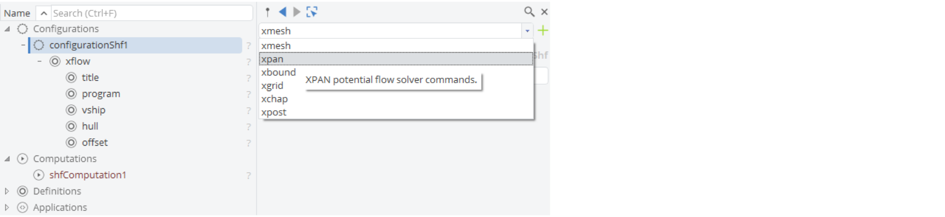
- Select “configurationShf1” and add xpan to the configuration.
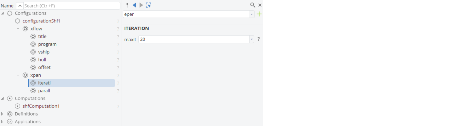
- Select xpan and set the maximum number of iterations to
20.
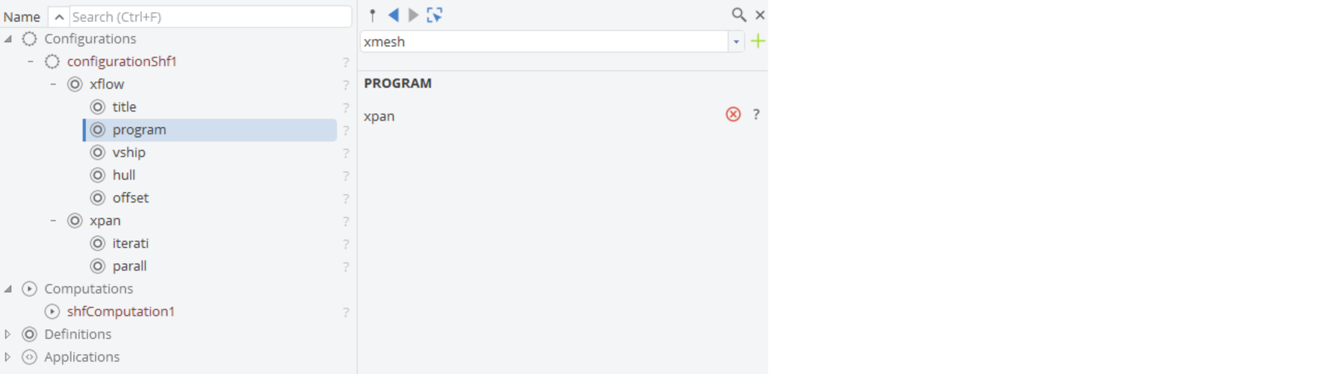
- Select the program entry of xflow in the tree and add xpan via the pull-down menu again. This activates the potential flow analysis.
SHIPFLOW Computation
The setup is ready now. The last step before running the potential flow analysis is specifying the computation i.e. the object which controls the SHIPFLOW executable.
-
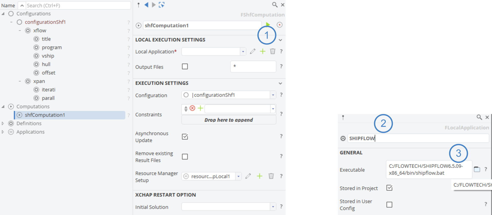
Select the computation “shfComputation1” and add a new local application. (1)
-
Set a meaningful name for the application such as “SHIPFLOW”. (2)
-
Set the path to your file
shipflow.batfrom the SHIPFLOW installation path. (3) -
Close the editor of the local application so that only “shfComputation1” is given and selected.
Make sure that finally the new local application is chosen from the pull-down menu.
Run and Monitor SHIPFLOW
The configuration is ready as well as the computation. Let’s run SHIPFLOW for the given geometry:
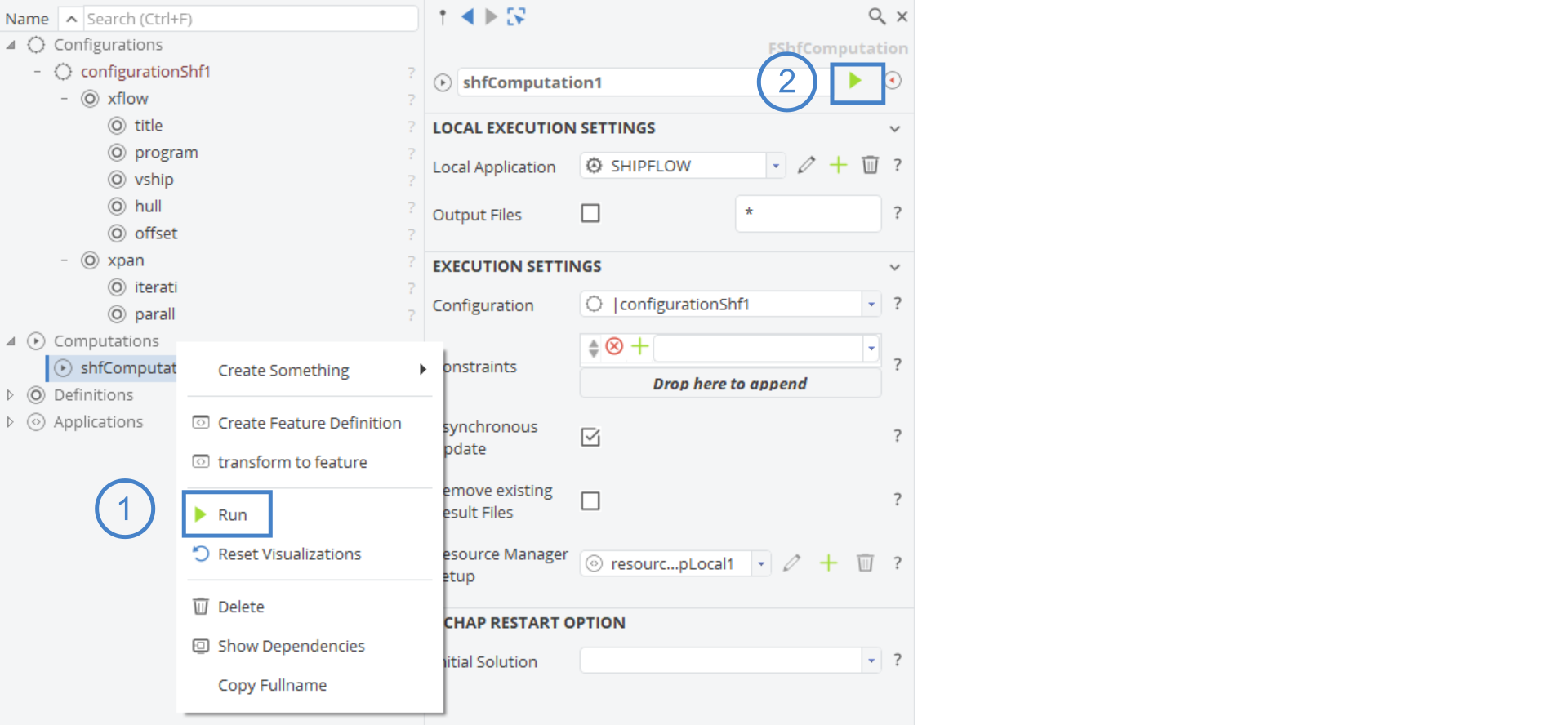
- Select “Run” from the context menu of the computation (1) or from the objectEditor (2).
The console output of SHIPFLOW can be monitored via the “TaskMonitor” widget which is located at the right-hand side of the user interface.
- Choose Menu > View > Windows > TaskMonitor (1)
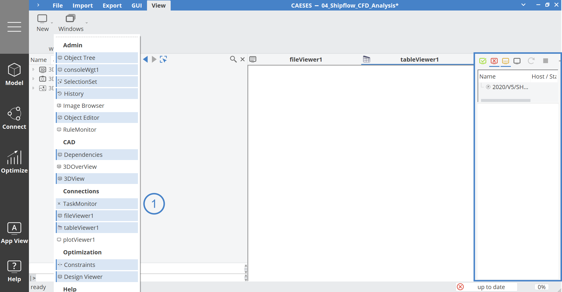
It shows the singular steps of calculation, such as preparing the offset path, creating offset groups for SHIPFLOW and running 20 iterations of XPAN.
Post-Processing
CAESES allows post-processing of SHIPFLOW results. Calculation results (several flow and resistance coefficients etc.) are provided as well as interactive visualization of the simulation. Please note that there is a separate tutorial for general post-processing. As a summary, the most important things to know are:
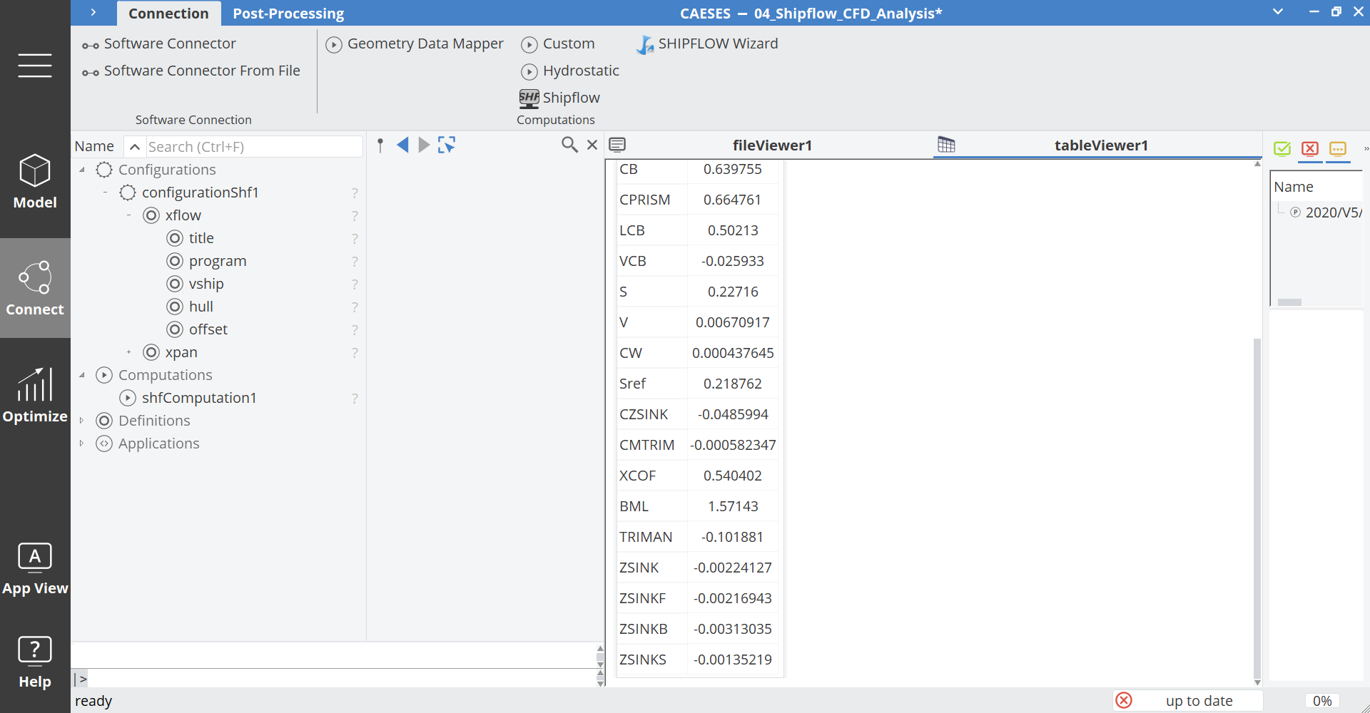
- The “TableViewer” widget shows the key result values from the analysis. In order to extract a table value, double-click on a single table item: A parameter gets automatically created in the tree (Model) which monitors this value.
-
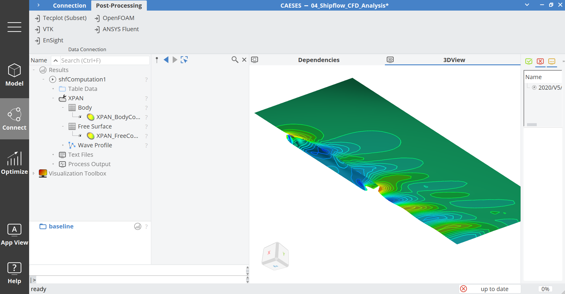
The visual results such as wave heights of the potential CFD calculation can be observed in the 3D view.
-
All results can be accessed and configured in the tree of Connect > Post-Processing > Results. In this case, all XPAN data is available in the XPAN scope of “shfComputation1”.
CAESES Project File
If you want to take a look at the finalized parametric model you can find the resulting CAESES project file shipflow-connection.cdb here: