Buttock-Based Aftship
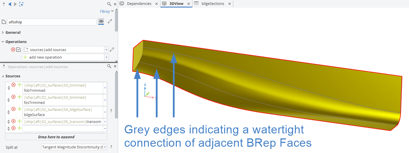
 This section covers the details of modeling a fully parametric bare aft body based on buttocks, which is part of the Component-Based Ship model within the Ship Modeling Workflow. The screenshot above shows a possible resulting hull combination including an integrated single skeg.
To follow this guide, a Component-Based Ship can be created inside a blank CAESES project. A set of hull parameters and the buttock-based aftship are all that is needed.
Introduction
Let's get started by taking a look at the provided scope structure and Design Variables. From the Model > Maritime tab choose a new Component-Based ship and create a set of Hull Parameters:
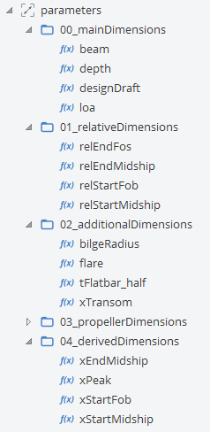
The main dimensions of the hull are given in parameters|00_mainDimensions as absolute values beam, depth, designDraft and length over all (LOA) in [m]. Although the model focuses on the aft body, its dimensions are derived from the overall ship dimensions.
Similarly, even when no flat bar (also known as flat iron) will be applied along the length of the keel, it is helpful to keep this option available by introducing the parameter tFlatbar_half from the very beginning of the modeling (see Scope 02_additionalDimensions). It can always be set to a value of zero at a later stage. The absolute x position of the transom is also given here as xTransom. In addition, flare and bilgeRadius are introduced to ensure connectivity towards mid- and foreship.
In 01_relativeDimensions, relStartMidship and relStartFOB are specified. They are given as a fraction of LOA as is the case for the additional values provided in the same scope.
One of the fundamental concepts in parametric modeling is to keep things dependent on each other. This way, even large variations in shape will result in valid geometries. One easy way to achieve this is to set up design variables as a fraction of the main particulars. When using these values during the modeling, their actual absolute measures need to be calculated by multiplying with the reference length (in Scope 04_derivedDimensions a few commonly used absolute values are stored for convenience).
Geometry Curves
To offer a simple access to the shape properties, three curves are defined. These curves are the transom shape, the lower limit of the flat of side (FOS) and the flat of bottom (FOB). These curves are linked to the main dimensions of the hull and parameterized in a way that allows a wide variety of shapes to be generated without generating a large amount of infeasible shapes. The user is free to approach this differently or add additional degrees of freedom if the default configuration does not solve a particular design requirement.
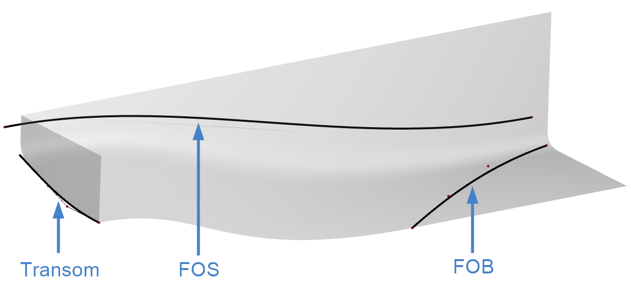
In the given configuration, the transom of the hull is described as follows: 4 points are located at xTransom starting from the center plane towards the FOS. The height (as a fraction of mainDimensions|depth) of the start and end point is linked to the Design Variables relZstart and relZend, respectively. The outer point marks a virtual bilge, i.e. if it was a hard chine and no curved bilge was used. For the start tangent, the deadrise angle can be modified, the end tangent can be offset via dAngleEnd from a natural angle that is defined by the additional construction line forTangent. The resulting design space stays within the correct range of the overall dimensions of the hull while allowing freedom such as a tunnel or v-shaped sections.

Since the FOS is linked to the transom curve, it can already be seen changing its absolute height at the start. In addition, the start angle, as well as the bilge radius (defining the z coordinate at the end) can be used as independent Design Variables. The curve is modeled as an F-Spline, hence further options to control the shape are naturally available but not exploited in the default set up of the model. Again, a different type of curve may be introduced as per the user's requirements. Finally, the FOB is again modeled as a B-Spline curve from 4 control points. The start position is linked to the relStartFOB parameter, other variations such as changes in main dimensions are not shown in the animation to not distract from the detailed shape changes.

Initial FOB and FOS Surfaces
The construction of the buttock based aft body is made of three surfaces. The concept of this model is, to set up the hull as a hard chine hull initially. The bilge radius is then added at a later stage after trimming the initial surfaces. One Meta Surface defines the bare (untrimmed) Flat of Bottom (FOB), a Ruled Surface the bare (untrimmed) Flat of Side (FOS) and another Meta Surface connects the actual FOB and FOS as a bilge surface.
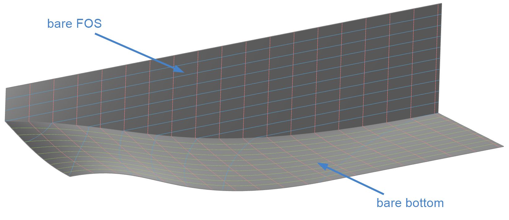
The key element for the initial hard chine hull is the bareBottom surface which connects the transom to the parallel midship of the hull. This is achieved via a Meta Surface that lofts buttocks from the center plane towards the FOS. Hence, this modeling approach is referred to as buttock-based.
The Curve Engine forButtocks defines each buttock such that it starts from the transom at a given angle and connects to the FOB curve at a horizontal angle. From there it follows a straight line to the parallel mid.

As in many fully parametric models, the basis for the final geometry is a set of defining curves. These curves may be geometric features such as the above mentioned transom, FOS and FOB but may also represent parametric values such as the buttock angle at the transom as a function of beam. The buttock at the center plane can be chosen freely. The function then defines the angle distribution along the y-axis towards the FOS where it needs to match the FOS curves shape. In this guide we have limited the number of functions to the most important ones, allowing the user to add more functions as an exercise or as per design requirements.
Paying close attention to these curves and the way they are parameterized is crucial.
Trimming
Once the two surfaces are established, the next step involves trimming them to create a bilge surface that connects them. Trimming is most effectively done using BReps (Boundary Representations). This method is ideal because BReps are specifically designed to trim NURBS surfaces using boundary curves in either 3D space or the UV parameter space of the surface. Importantly, this approach does not re-parameterize or approximate the original surfaces. For the trimming, the Project and Trim method is used and the resulting Faces are shown in the following screen shot:
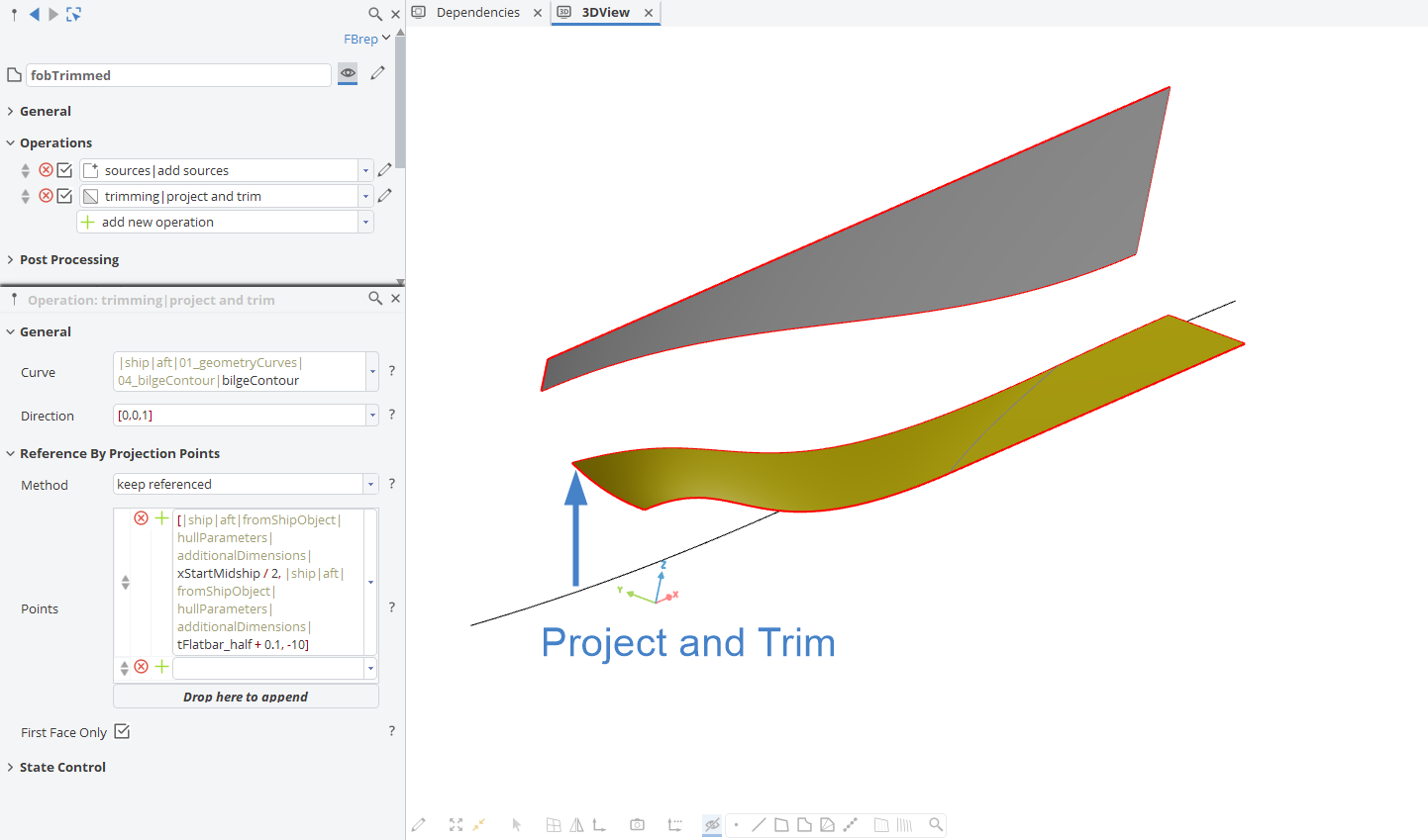
In order for the Project and Trim operation to work reliably in a parametric model, it is important to choose a reference point that works for all shape variations that are to be expected.
Bilge Surface
The bilge surface is created as a Meta Surface. It is lofted in longitudinal (x-) direction of the hull and modeled as a NURBS curve with 4 control points. The first and last point lie on the projected FOB and FOS contour curves, respectively. The two intermediate points are positioned such, that tangent continuity towards the two adjacent surfaces is ensured. This leaves one degree of freedom (the position along the tangent vector) which is referred to as "Tangent Speed" in the input arguments of the Curve Engine. In addition, the weight of the two intermediate control points can be varied.
To get a better understanding, a test section can be created temporarily by selecting the Curve Engine and typing the following command into the console:
.createFeature(parameter pos(0))
Changing the input arguments of the resulting feature will allow to get a good understanding of how they affect the shape of each individual section that makes up the final bilge surface.

To ensure the bilge connects smoothly to the parallel mid, the functions defining tangent factors and weights along the x-axis are designed to match the exact values of the mid-frame bilge. Additionally, their derivatives must be zero, as tangent factors and weights remain constant along the midship.
For the Meta Surface it is important to set both rails to ensure a watertight connection towards the trimmed FOB and FOS. The rails resulting from the trimming of the initial surfaces can be conveniently selected using the BRep Based > Edge or Tangent Edge curve type.
Transom Face and Final Combined Bare Aftship
Finally the transom is modeled. This is done via a Planar BRep Edge and a Faces from Planar Curves. The transom, trimmed FOB, FOS and bilge surface can now be joined into a final BRep.