CFD Results Comparison
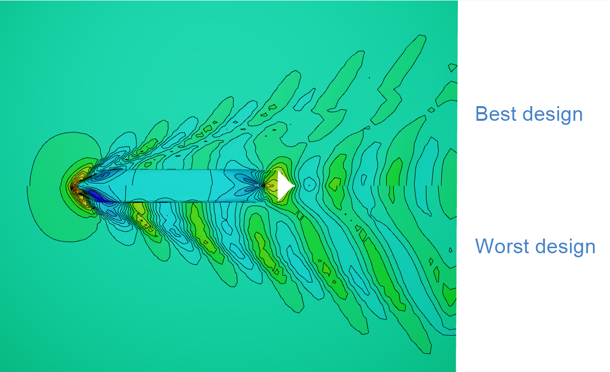
Comparing CFD results is commonly done by comparing the values of, e.g., the resistance or the propeller thrust and by a visual inspection of the resulting wave pattern or pressure distribution. This tutorial explains how to compare CFD results in the 3D view on the example of a variation of the default ship from the Ship Modeling Workflow which is evaluated using a simple SHIPFLOW setup.
Hull Model
As an example, we use the sample of the component-based ship which is a ship type of the Ship Modeling Workflow:
Get Started With Ship Hull ModelSince the offset generator in SHIPFLOW only handles half models without a deck or transom, we must adjust the output in the main dialog of the Ship Modeling Workflow accordingly.
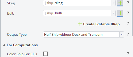
The result is a fully parametric and watertight ship model.

SHIPFLOW Setup
For this example, we use a simple and quick SHIPFLOW setup, using only potential flow (XPAN) with a fixed ship.
As a first step, we create a new SHIPFLOW setup in the Connect tab.
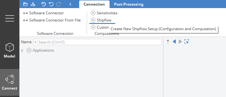
To make the setup functional, we have to add:
- The offset tab, including the geometry (stlf) and LPP (lpp)
- The ipos tab to set the trim (trim) and draft (tm)
- The ship speed (vknot) in the vship tab
The LPP can be measured to 237 m (as it is only used for reference to compute the Reynolds number and we are running potential flow computations, it does not have to be very accurate). For the geometry file (stlf) we use the output of the Ship Modeling Workflow and export it as STL file. In the xflow tab, we must add the stlf tab and insert |ship:ship.exportSTL("ship.stl"). The trim should be set to 0 and the draft to the design draft (10 m). As a ship speed, we can use 20 kn for this example. To save time, we can set the grid density (xmdens in hull) to coarse and we can limit the number of iterations in XPAN-control-iterati-maxit to, e.g., 10 and even set the model to be fixed.
The final SHIPFLOW setup should look like in the picture below.
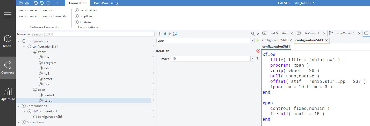
In the SHIPFLOW computation, we must add the application (this tutorial is tested with SHIPFLOW 8.0). Make sure to adjust the maximum number of running instances according to your computer’s performance.
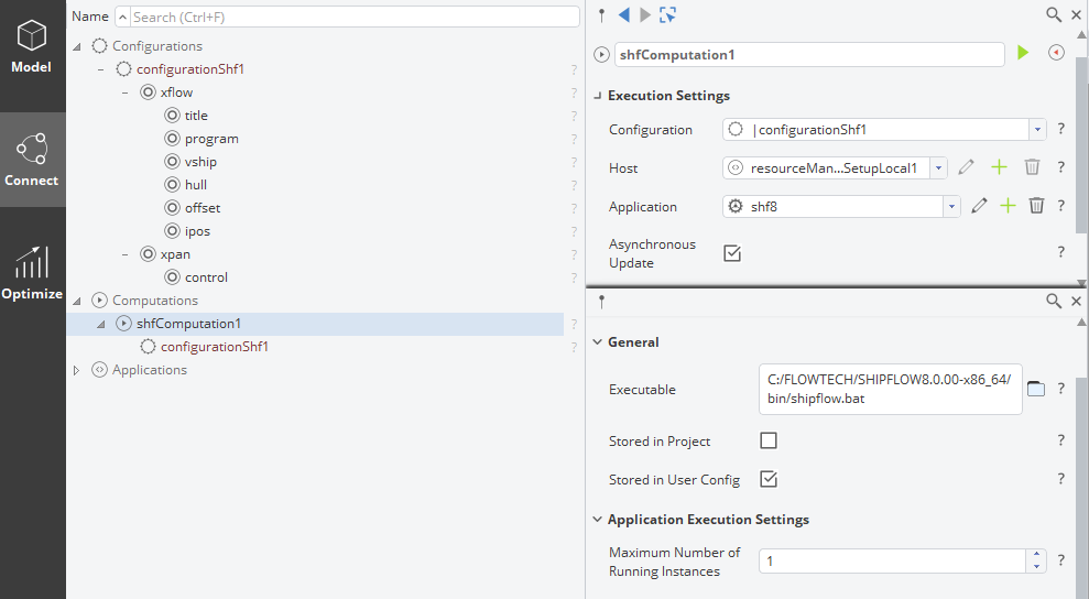
The SHIPFLOW setup should now be ready for a test run. To access the results parameters, double click on the value in the table viewer, which will automatically create a parameter. For the later variation, we will use the wave making resistance CW.
Variation
Since we want to compare different variants of the hull, we must use a simple variation. For this tutorial, we use a SOBOL with two variables and the wave making resistance as monitored evaluation. Two variables with significant influence on the wave pattern are the bulb length (|ship|bulb|01_geometryCurves|03_contour|relBulbLength) and the end of the parallel midship (|ship|parameters|01_relativeDimensions|relEndMidship). The final setup of the SOBOL should look like in the picture below.
The boundaries of the design variables have been adjusted for larger variation in the results.
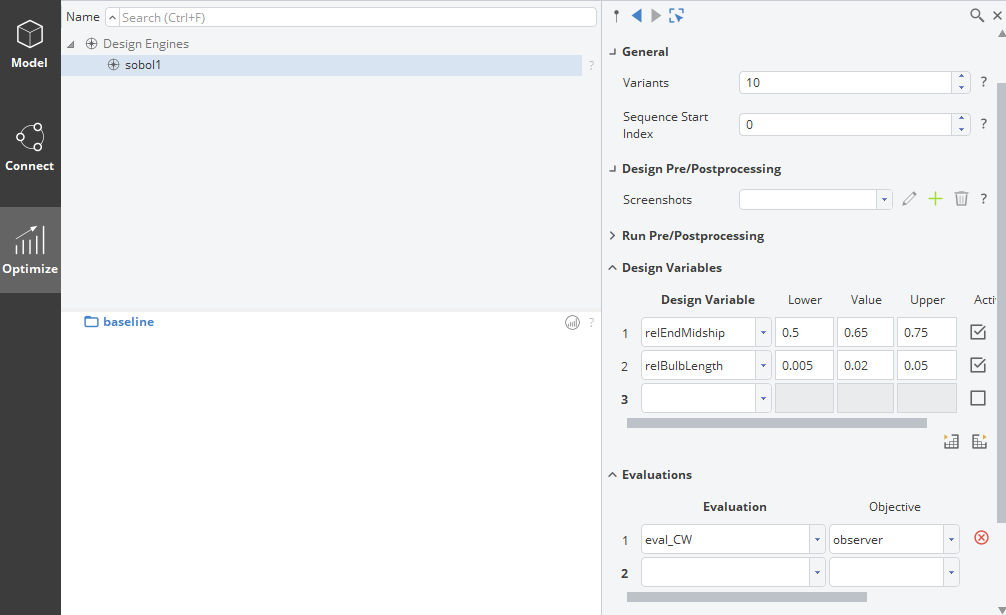
Now it is time to run the variation and wait for the computations to finish.
Results Comparison
Analyzing and comparing results can be done (among others) by viewing charts of the evaluated parameters and constraints over the design variables or by visually comparing the resulting wave patterns and pressure distributions,
Charts
To view the charts, navigate to the Optimize tab and select the relevant results table. On the top left you will notice a button View Charts.
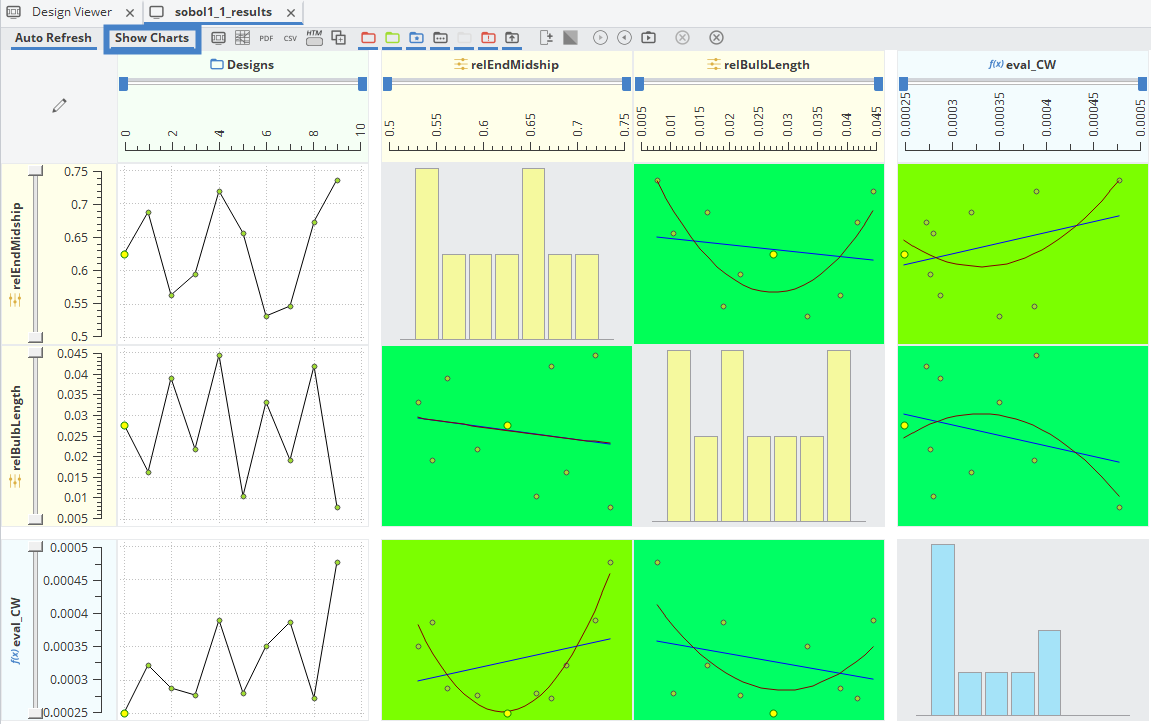
From this analysis of our results, we can conclude a very clear dependency of the wave making resistance on the forward end of the midship, with a clear optimum at around 0.625. The trends for the bulb are not as pronounced, but lower resistance values are achieved with longer bulbs.
3D View
To view results in the 3D view, navigate to the Connect tab and select Post processing. Here you can also modify the appearance of the results by adjusting the color scheme, creating or selecting a color map or adding black line in between the different colors. It is favorable to always use a fixed color map to better judge the differences between the hulls. Automatically colored results will make a fair comparison more difficult.
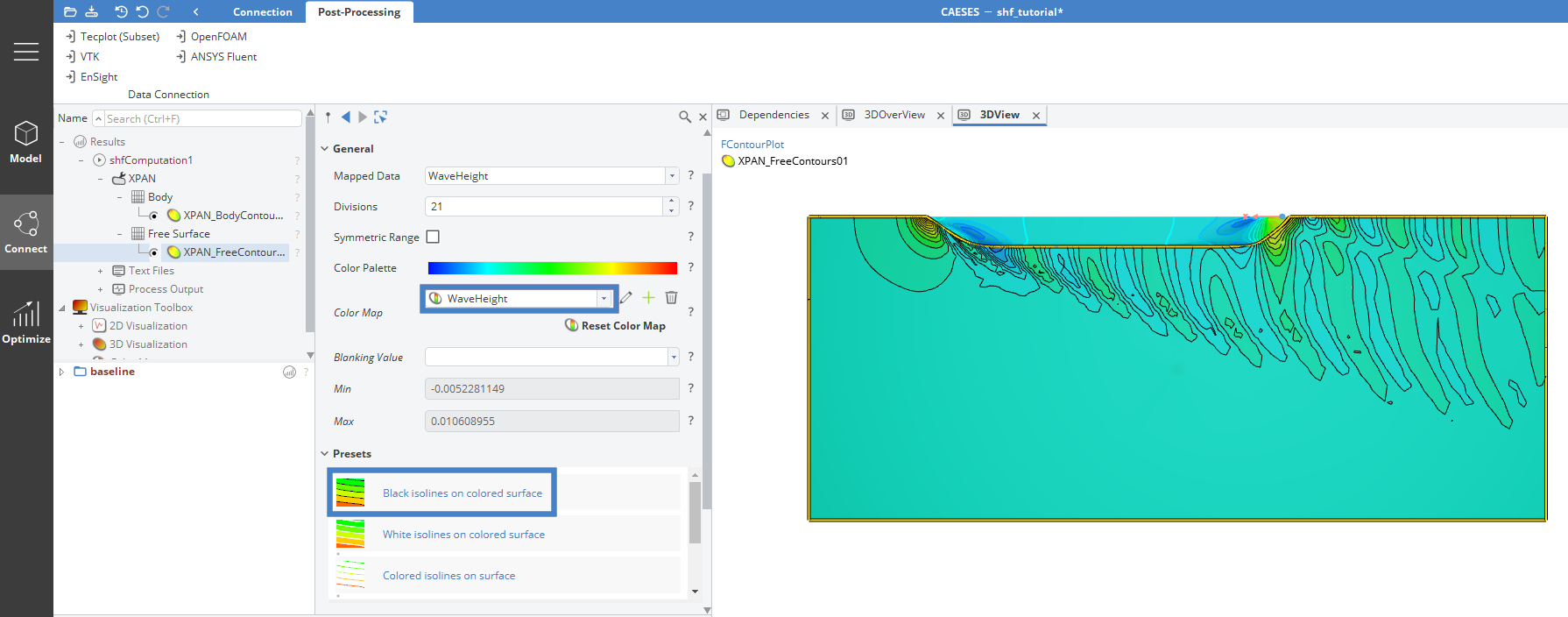
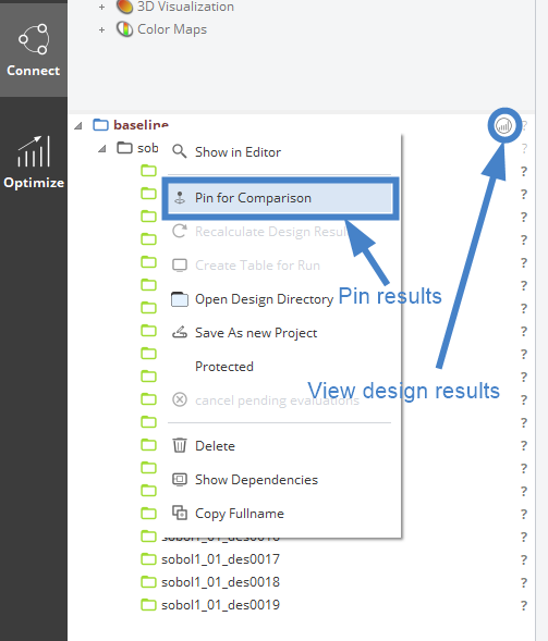
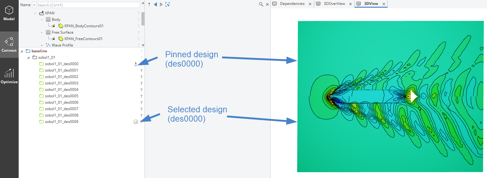
To compare different variants, the results of a variant can be pinned. Right click on the variant that shall be pinned and select Pin for comparison. The pinned results will be mirrored and stay there, no matter what design is selected. To view the results of other designs, click on the icon to the right of the design name in question.
Make sure to disable mirroring in the 3D View, otherwise the pinned and the selected results will be on top of each other.
With these settings, different designs and their results can easily be compared.
CAESES Project File
The final CAESES project file (without results) cfd-results-comparison-shipflow.cdb can be found here: