Maxsurf Connection

MaritimeThis functionality requires the Maritime add-on to be enabled. 5.3.0This functionality requires CAESES version 5.3.0 or later.

This tutorial guides you through connecting Maxsurf software with CAESES. Maxsurf offers various tools for different applications and this tutorial focuses on two key functionalities:

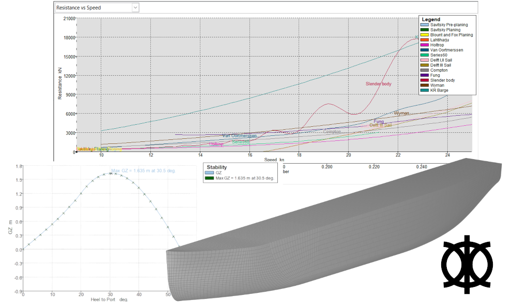
Maxsurf Stability and Maxsurf Resistance leverage Component Object Model (COM) features from CAESES for their respective purposes:

• Maxsurf Stability: Performs intact stability calculations

• Maxsurf Resistance: Analyzes bare hull resistance

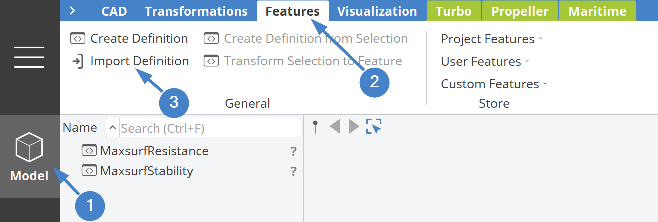
• Click the buttons below to load the feature definitions (in CAESES they are automatically added to your project).

Load Maxsurf Stability Feature Load Maxsurf Resistance Feature

If you downloaded the features to your computer you can import them using:

• Drag and drop to import the definitions into the CAESES project file or
• Alternatively, navigate to the Model workspace > Features tab, select Import Features and import the corresponding files.

For both connections, a panel mesh of the hull geometry is required, as shown in the image below.

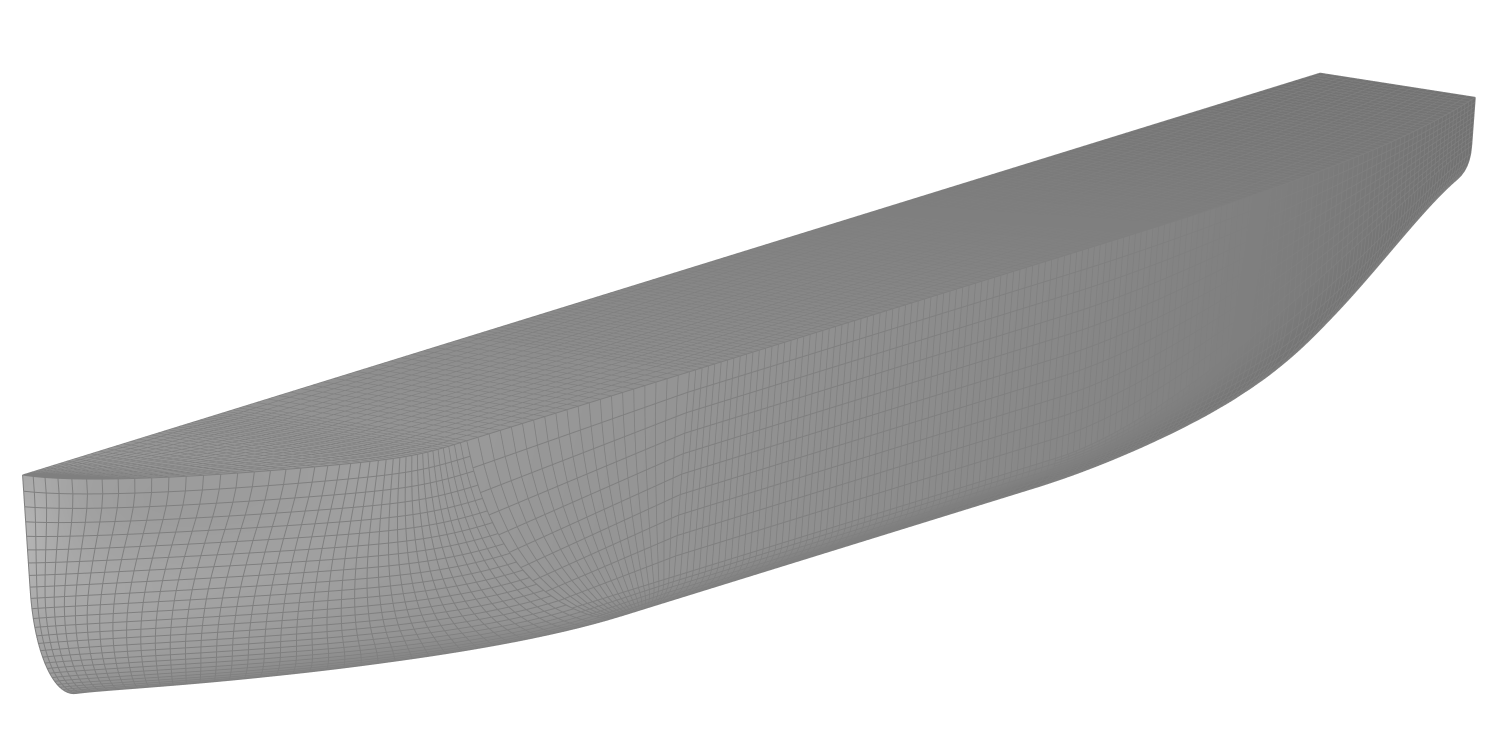
Ship Hull Model

The ship model used in this tutorial is generated from the Ship Modeling Workflow. It is essentially the default parameterized model from the component-based ship, without a bulb or a skeg and with properties defined by the Ship Object in CAESES.

• Create a Component-based Ship from the Model workspace > Maritime tab > Ship > Component-based

• Click the plus buttons in the Ship Object editor to add the:
  • Hull Parameters
  • Midship
  • Section-based Aftship
  • Waterline-based Foreship

This simple ship model will serve as a starting point for the Maxsurf connection.

Conditions

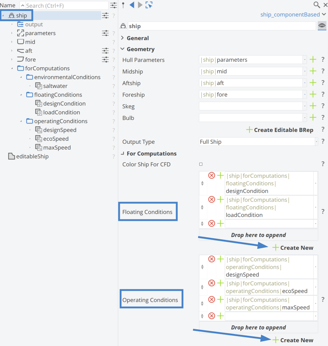
In the Ship Object in the category For Computations, two types of conditions can be defined, which we will set up in the next steps: Floating or Operating Conditions.

Floating Conditions

The default Floating Condition generated with the Ship Object is the designCondition, with the Prescribe Floating Condition checkbox enabled. Let's create another floating condition:

To create a new Floating Condition named "loadCondition":

1. Click the Create New button under Floating Conditions in the For Computations category of the Ship Object (the Prescribe Floating Condition checkbox is disabled per default for new floating conditions).
2. Rename the newFloatingCondition to "loadCondition"
3. In the newly created loadCondition add the saltwater environmental condition by choosing it from the drop down in the field Environment Condition
4. Click on the plus (+) button next to the Loadcase field to create a new load case
5. Rename the newLoadCase to "FLD"

info

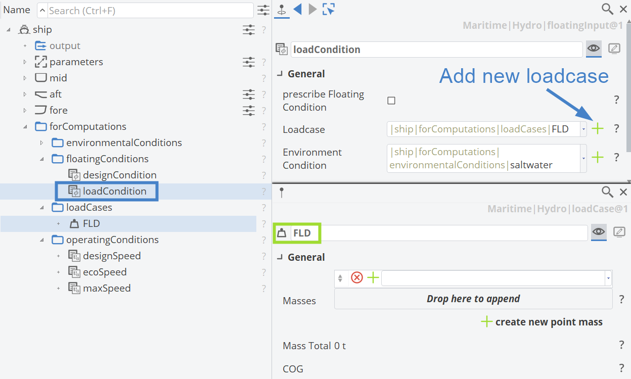
The abbreviation FLD stands for the ship at Full Load Departure, meaning it is fully loaded when leaving the port.

Defining Point Masses for a Load Case

Let's add two different Point Masses to the FLD loadcase. A Point Mass requires an input for the mass (in tons) and the center of gravity [as a vector].

LightShip (Weight and center of gravity of the ship without cargo):

• Select the FLD loadcase in the scope |ship|forComputations|loadCases
• Click the button "+ create new point mass"
• Rename the point mass to "Lightship"
• Set the Mass to 30000 t
• Set the Center Point (center of gravity) to

  [|ship.getHullParameters().getLoa() * 0.48, 0, |ship.getHullParameters().getDepth() * 0.7]  

Cargo (Weight and center of gravity of the cargo):

• Select the FLD loadcase in the scope |ship|forComputations|loadCases
• Click the button "+ create new point mass"
• Rename the point mass to "Cargo"
• Set the Mass to 70000 t
• Set the Center Point (center of gravity) to

  [|ship.getHullParameters().getLoa() * 0.49, 0, |ship.getHullParameters().getDepth() * 0.75]  

Total Mass and Center of Gravity

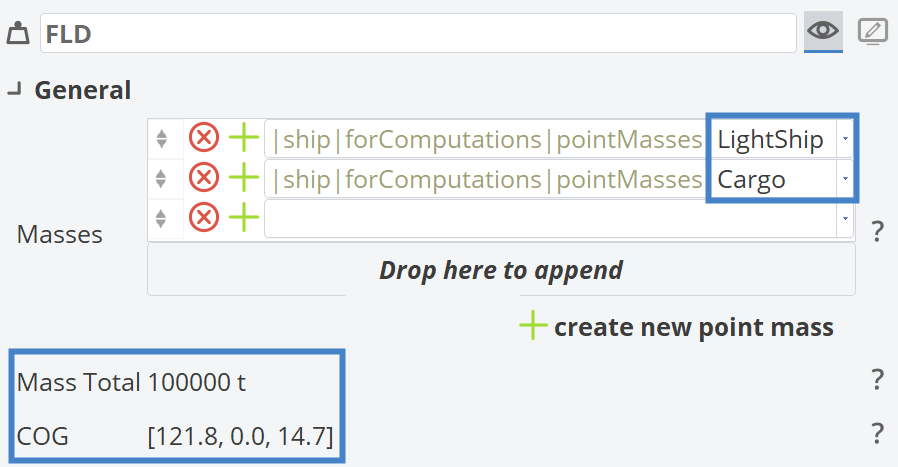
The Total Mass is displayed in the FLD loadcase and sums up to 100000 tons, with a Center of Gravity (COG) at [121.8, 0, 14.7] for the default parameterization:

Operating Conditions

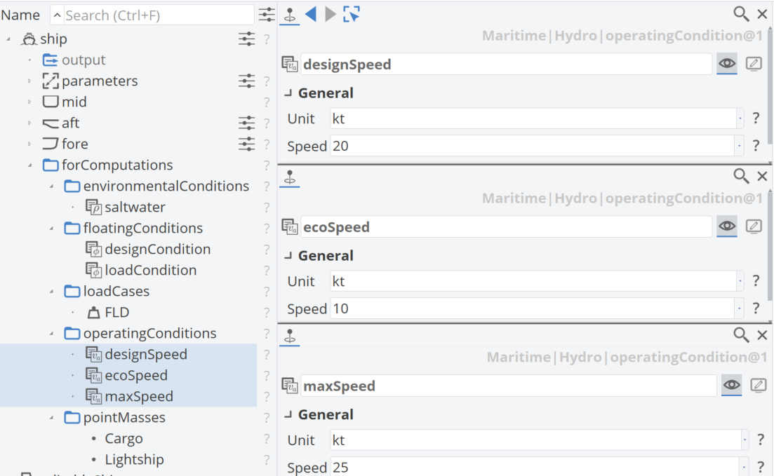
• Add three different Operating Conditions for the Ship Object by clicking the "+ Create New" button below the Operating Conditions list.
  • Rename the first newOperatingCondition to "designSpeed" and set the value to 20 kt
  • Rename the second newOperatingCondition to "ecoSpeed" and set the value to 10 kt
  • Rename the third newOperatingCondition to "maxSpeed" and set the value to 25 kt

Surface Patches

Once the setup of the Ship Object is finalized, click the Plus Button next to Create Editable BRep. This generates a BRep named editableShip with the source ship:ship, which returns the BRep geometry of the Ship Object that was created.

Next, follow these steps:

• Create a scope named "00_surfaces" and add the generated BRep editableShip to this scope via drag and drop.
• Create three subscopes under 00_surfaces:
  • "00_aft"
  • "01_mid"
  • "02_fore"

The purpose of this setup is to organize all Surface Patches of the ship model within a single scope.
Generally, Image Surface will be used to import the appropriate BRep Face ID.

Aft Surface Patches

We want to pick a surface patch from the editableBRep and use it as an input for a new Image Surface:

• Make sure the editableShip object is visible in the 3D view (the scope that contains the object should be visible, too, indicated by a blue color)
• Hide the Ship Object by clicking on the icon
• Make the 00_surfaces|00_aft your working scope by clicking on the scope icon with the middle mouse button (the working scope gets a green scope icon)
• In the 3D view disable the section visualization with the filter option to hide the sections overlay on the editableBRep. This will help in selecting the right surface patches.

• Hover with the mouse over the editableBRep in the 3D view and press Ctrl + Alt to enter the sub-selection mode. This will allow you to pick the surface patch (or face) of a BRep.
• While the sub-selection mode is activated (the geometry is rendered in a light blue color), click on a surface patch (the selected patch is shown in yellow )
• While the face is selected, create an Image Surface via Model workspace > CAD tab > Surface > Surface Based > Image. This will automatically set the selected surface patch as an input for our image surface.
• Set a name for the new image surface.

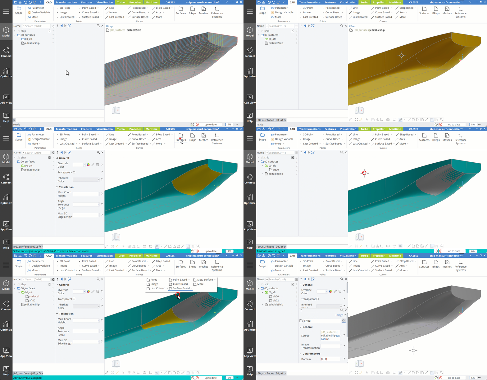
• Repeat the previous steps for all surface patches of the aft until every aft patch is included in an image surface

tip

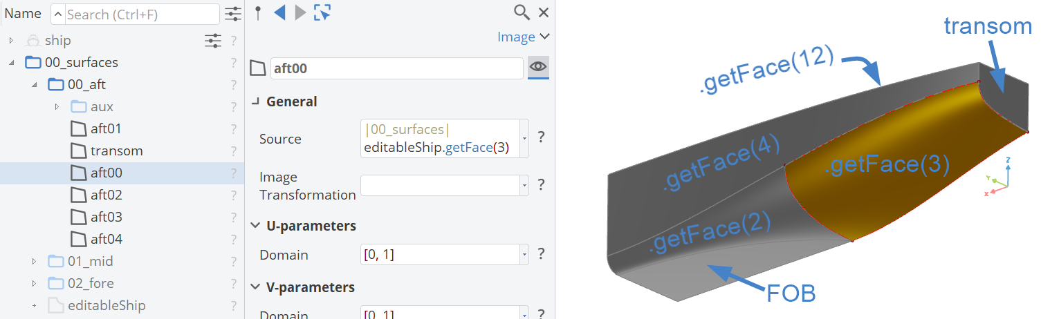
The sub-selection mode can be escaped by pressing Ctrl + Alt again.

However, two specific Surface Patches require specialized handling:

• Transom
• Flat of Bottom (FOB) in the aft body region

info

An Image Surface will not work in this case because some trimmed NURBS surfaces are used in the Ship Object, which prevents the Image Surface from accurately capturing the geometry. The Image Surface of a BRep Face will always include the untrimmed underlying NURBS surface.

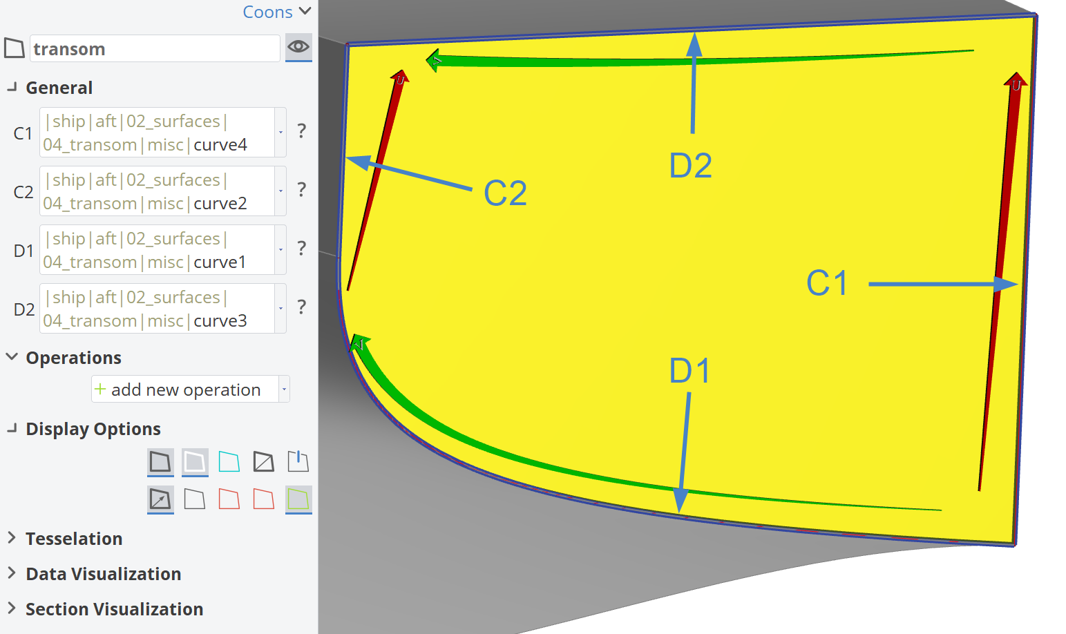
For the transom and flat of bottom surfaces, a Coons Patch will be used instead of an Image Surface, utilizing the Boundary Curves of the respective patches.

• Create a Coons Patch via Model workspace > CAD tab > Surfaces > Curve Based > Coons
• Set the input curves according to the screenshot below for the Transom.

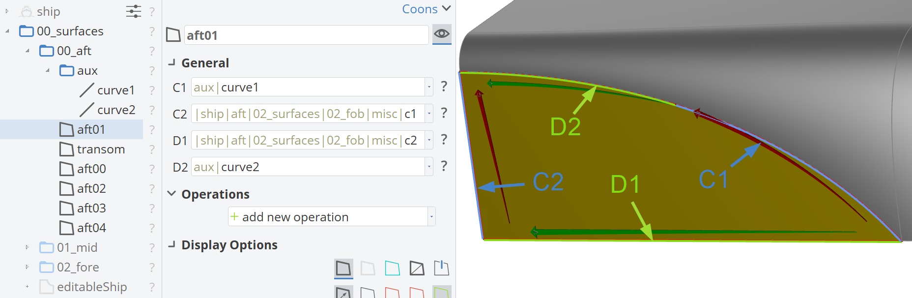
For the FOB in the aft body region, a Coons Patch named aft01 will be created.
The Ship Object provides three boundary curves under |ship|aft|02_surfaces|02_fob|misc|:

• c0
• c1
• c2

Since a Coons Patch requires four curves, additional Image Curves will be created:

• Create a new subscope under 00_aft and name it "aux"
• Create an Image Curve under aux and name it curve1, with the following properties:
  • Source: |ship|aft|02_surfaces|02_fob|misc|c0
  • Domain: [0.5,0]
• Create an Image Curve under "aux" and name it curve2, with the following properties:
  • Source: |ship|aft|02_surfaces|02_fob|misc|c0
  • Domain: [0.5,1]
• Set the input curves according to the screenshot below for the aft01.

All surface patches for the aft-body will be placed in the scope "00_aft".

Mid Surface Patches

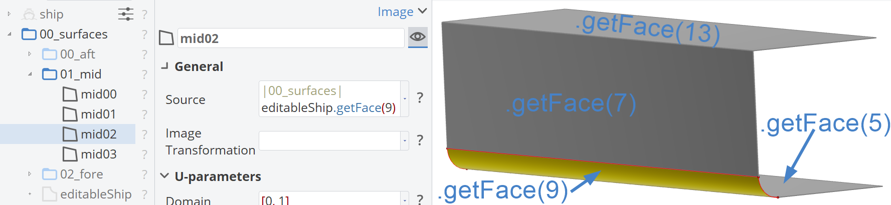
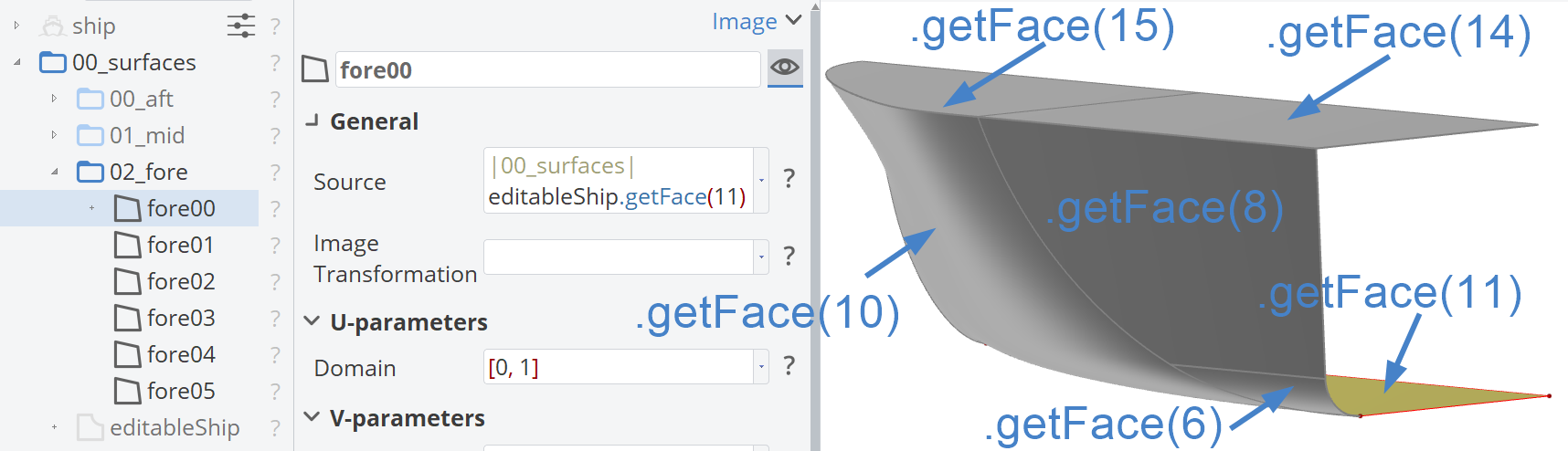
Following the same approach as used for the aft surface patches , we extract a surface patch from editableBRep and use it as input for a new Image Surface for the mid-body.
These patches will be placed in the 01_mid scope.

Fore Surface Patches

Finally, we extract the surface patches from editableBRep (just like it is shown for the aft surface patches) and use it as input for a new Image Surface for the fore-body.
These patches will be placed in the "02_fore" scope.

Panel Meshes

After collecting all the Surface Patches, the corresponding Panel Meshes can be created.

• Create a scope named "01_meshes" with the following subscopes:
  • "00_aft"
  • "01_mid"
  • "02_fore"

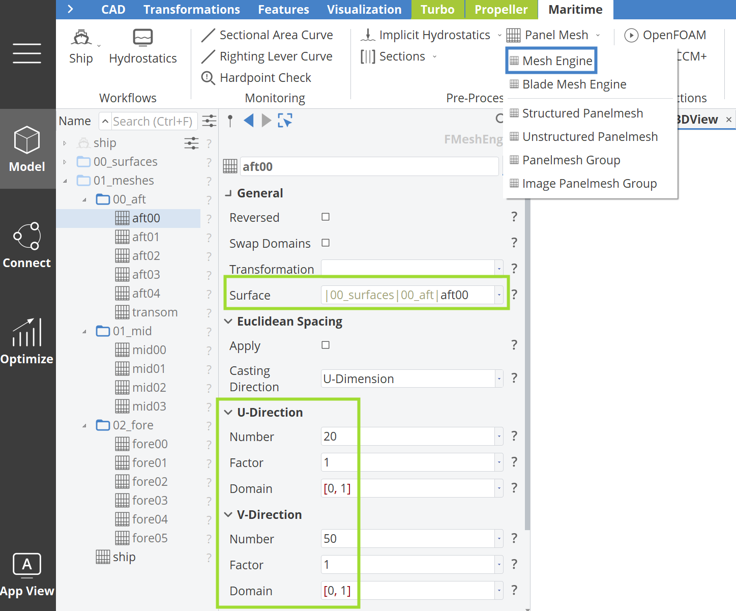
The Panel Meshes use the Mesh Engine object, which can be found under the Maritime Tab > Pre-Processing category > Panel Mesh > Mesh Engine. The Mesh Engine requires the following inputs:

• Surface Input
• Number of Panels in U-Direction
• Factor in U-direction
• Number of Panels in V-Direction
• Factor in V-Direction

Rational values for the factors range between [0.5, 1.5]:

• A factor of 1 provides a linear panel distribution.
• A factor > 1 concentrates more panels at the start of the U or V parametric domain.
• A factor < 1 concentrates more panels at the end of the U or V parametric domain.

For this tutorial:

• All factors should be set to 1.
• The parametric domain in both directions should cover the entire range [0,1].

Click to expand: Number of Panels in U & V-Direction for each Panel Mesh

Name	U-Panels	V-Panels
aft00	20	50
aft01	20	20
aft02	20	40
aft03	10	80
aft04	20	80
transom	10	20
mid00	20	60
mid01	10	60
mid02	10	60
mid03	20	60
fore00	10	40
fore01	10	20
fore02	10	20
fore03	20	20
fore04	20	40
fore05	30	40

tip

The goal when creating the panel mesh is to achieve quadrilateral elements with an aspect ratio as close to 1 as possible (i.e., square-shaped panels).
However, achieving this perfectly is not always possible. Users should adjust the panel mesh inputs based on the curvature of the surface.

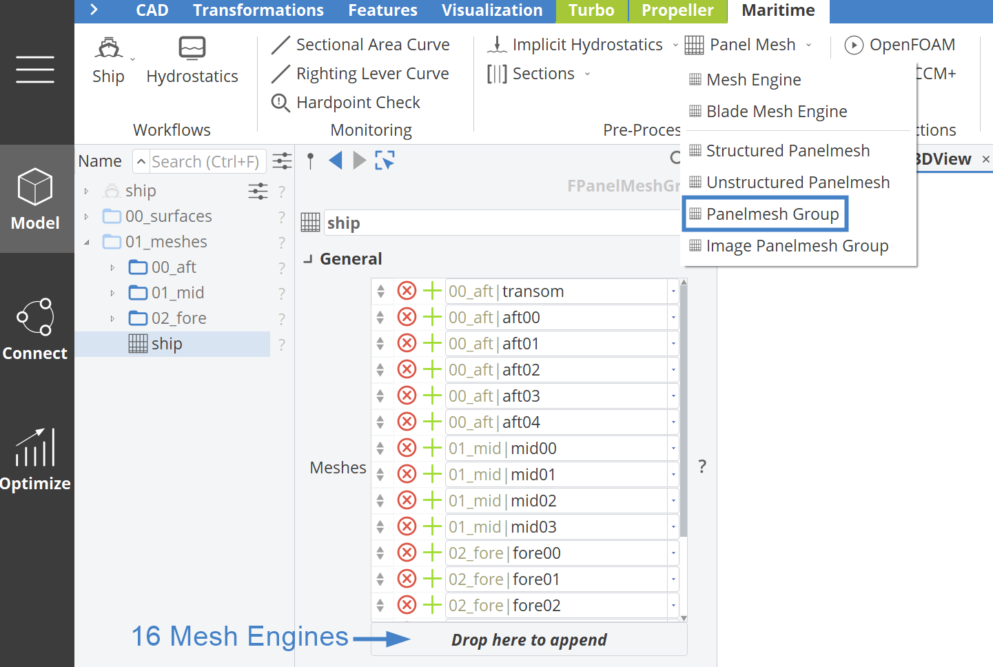
In the end, all the collected Panel Meshes should be grouped into a Panel Mesh Group named ship, containing 16 entries in this tutorial.

Maxsurf Stability

For this tutorial we will perform an Intact Stability Calculation by running the Maxsurf Stability software from CAESES. The input for the Feature is shown in the figure below.

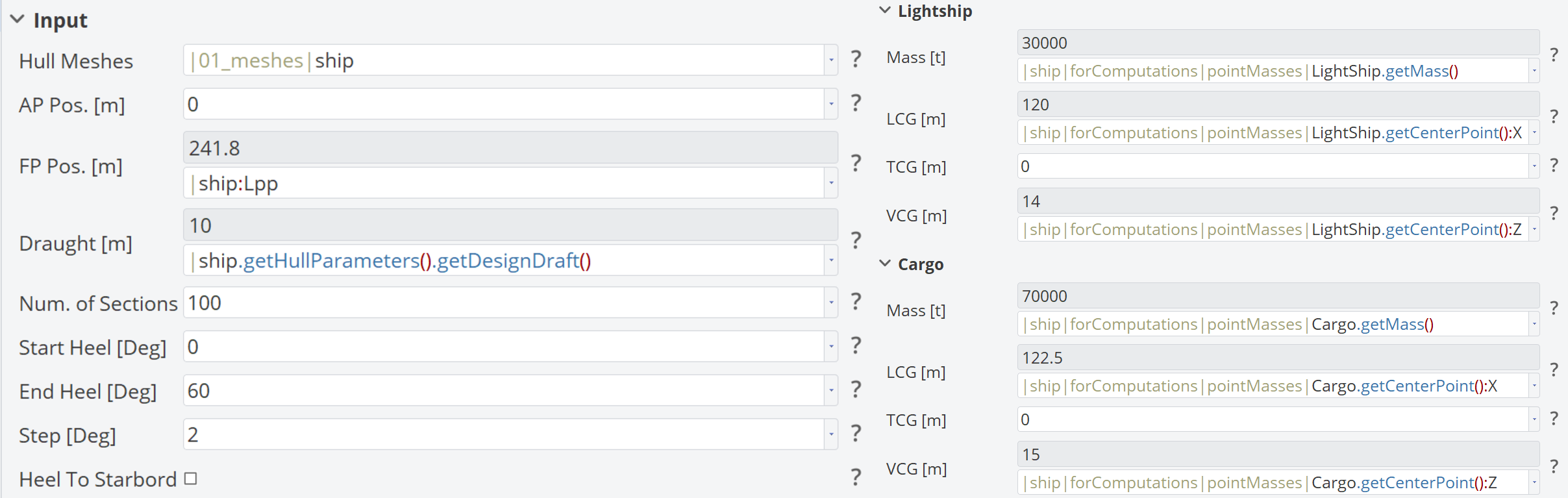
The Hull Meshes provide the ship geometry that we created and are linked to the parametric model we constructed.
The Aft & Fore Perpendicular Positions and Draught can be obtained from the Ship Object.

Stability Calculation Parameters

• Number of Sections: Defines the number of sections used for hull generation in Maxsurf. A value of 100 is recommended, with a maximum of 200.
• Start & End Heel (degrees): Defines the heel angles for calculating the GZ curve.
• Step: Specifies the interval between each heel value. For example, a step of 2° results in calculations at 0°, 2°, ..., 60°.
• Heel to Starboard Side: An optional setting; by default, calculations are performed on the Port Side.

Mass & Center of Gravity

Apart from these inputs, the Lightship & Cargo weights (in tons) and their respective Centers of Gravity (in meters) must be provided.
These values can be obtained from the Ship Object, as illustrated in the figure above.

note

The abbreviations in the input of the Feature LCG, TCG and VCG stand for Longitudinal (X-axis), Transversal (Y-axis) and Vertical (Z-axis) Center of Gravity.

Stability Calculation Outputs

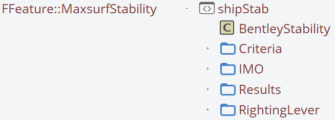
In CAESES, four different scopes are generated under FFeature::MaxsurfStability:

• Results: Contains vectors of doubles (FDoubleSeries) for the given Heel Angles and various Hydrostatic parameters.
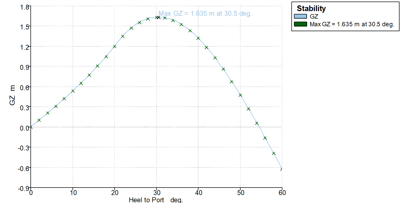
• Righting Lever: Stores the Righting Lever Curve (3rd Degree Interpolation Curve), representing GZ (in meters) versus Heel (in degrees).
• IMO: Includes double parameters used to check the IMO Criteria for Intact Stability, retrieved from the Righting Lever Curve.
• Criteria: Boolean parameters that determine whether the IMO Criteria are met (true) or violated (false).

Additionally, the COM Object responsible for calling the software, named BentleyStability is provided as an output of the Feature.

When Maxsurf Stability is executed from CAESES via the provided Feature, a Word report and a hull_Report.txt file (located in the corresponding Project Directory of the CAESES project) are automatically generated.
Below is the GZ curve (Righting Lever Curve) for the generated Ship Object, displaying values from 0° to 60° and checking compliance with all IMO Criteria.

Maxsurf Resistance

For this tutorial, as mentioned earlier, we will perform a Bare Hull Resistance Calculation by running the Maxsurf Resistance software from CAESES. The input for the Feature is shown in the figure below.

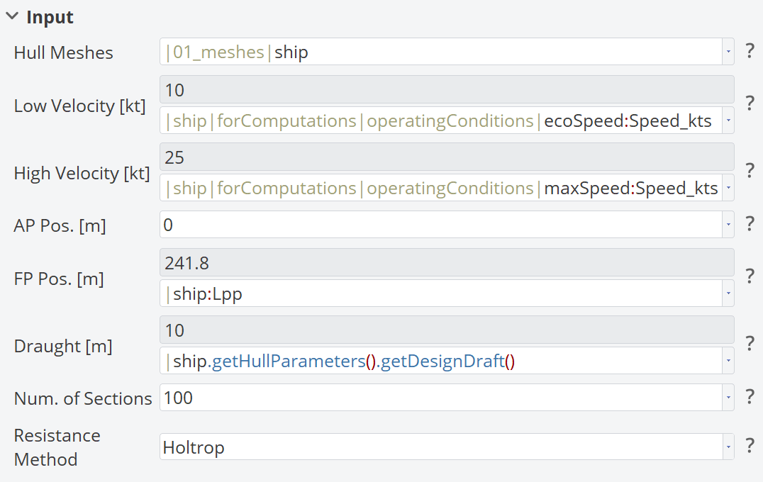
Similar to the Maxsurf Stability process, the Hull Meshes, Aft & Fore Perpendicular Positions, Draught and Number of Sections are provided.

Resistance Calculation Parameters

The resistance in Newtons will be computed for a range of speeds, given in knots. You need to provide the lowest and highest velocity, which can be retrieved from the Ship Object, as we have already defined the Operating Conditions.

Additionally, the Resistance Method is selected from a list of potential options available in Maxsurf. Below is the categorized list of these methods, with a small comment for each one:

• Planing Hulls:

  • Savitsky Pre-Planing: Used for estimating resistance in the pre-planing phase of a hull.
  • Savitsky Planing: Used for predicting resistance in the planing phase of a hull.
  • Blount and Fox Planing: Another method for predicting resistance in planing hulls.
  • Lahtiharju: A method for estimating resistance in planing hulls at high speeds.
  • Wyman: An empirical method for resistance prediction in planing hulls.

• Displacement Hulls:

  • Holtrop: A widely used method for estimating resistance in displacement hulls.
  • Compton: An empirical method for calculating the resistance of displacement hulls.
  • Fung: A resistance prediction method based on an analytical approach for displacement hulls.
  • Van Oortmerssen: An empirical formula used for resistance in displacement hulls.
  • Series 60: A series of empirical resistance prediction methods for displacement hulls.
  • KR Barge: A method used to predict resistance in barge-like hulls.

• Yachts Hulls::

  • Delft I, II Sail: A method for predicting resistance in yachts, primarily for sailboats.
  • Delft III Sail: Another method for sailboats with different assumptions and models.

• Analytical:

  • Slender Body: Used for predicting resistance of slender bodies, typically applied to long, narrow hulls.

For the Ship Object we have generated in this tutorial, we will use the Holtrop method, as it applies to a displacement vessel with a large LOA of 250 m and is widely used.

Resistance Calculation Outputs

In CAESES, two vectors of doubles (FDoubleSeries) are generated under FFeature::MaxsurfResistance:

• vel: Inflow velocities in knots, which will be used for the resistance calculation.
• Rt: Resistance force in Newtons for the various velocities given in knots, based on the chosen Resistance Method.

Additionally, the Feature generates a ResistanceResults.csv file (resResults under the Feature, which is an FFile object) in the corresponding Input Directory of the CAESES project. This file contains two columns: speed in knots and resistance in Newtons, corresponding to each value.

A Resistance Curve is also generated as a 3rd Degree Interpolation Curve, representing resistance in Newtons (N) versus velocity in knots (kt).

Finally, the COM Object responsible for calling the software, named BentleyResistance, is provided as an output of the Feature.

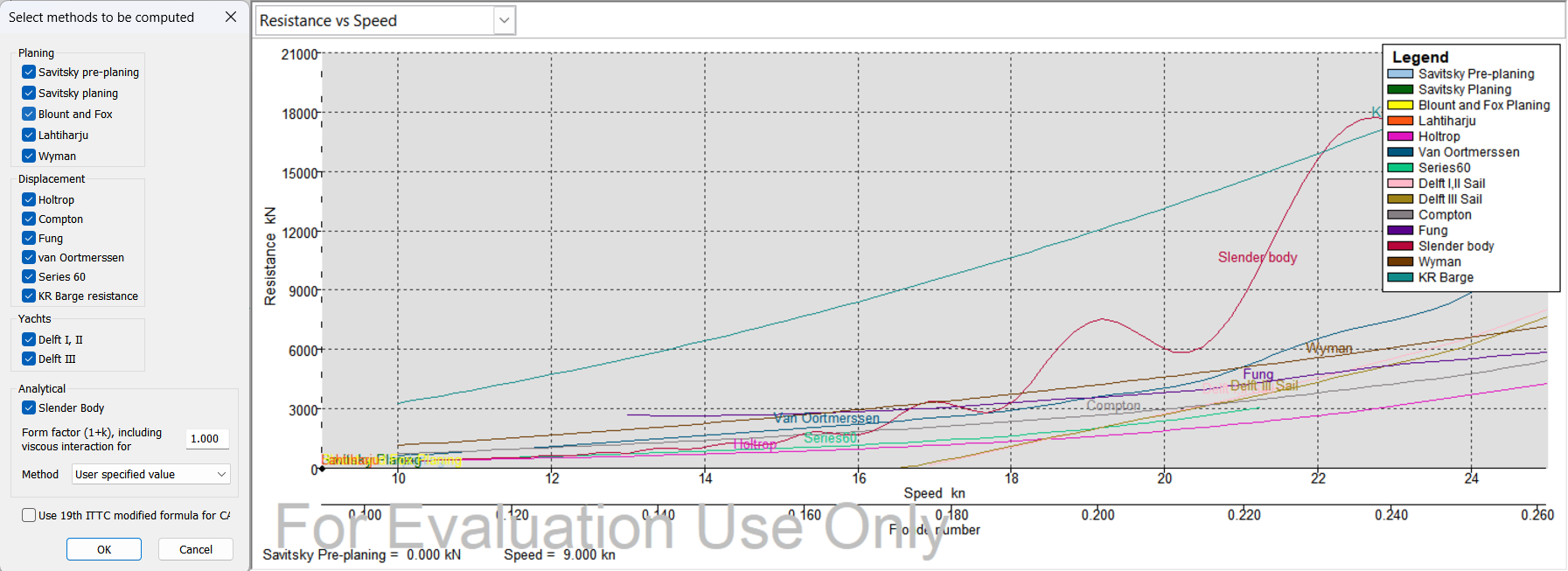
When Maxsurf Resistance is executed from CAESES via the provided Feature, all the Resistance Method calculations are plotted in the GUI of Maxsurf over the selected range of velocity speeds. This allows for a general overview of how different methods provide different results and which one fits best. However, in CAESES, only the chosen method from the Feature is returned as a result.

Conclusion

This tutorial showcases a sample ship hull model generated from the component-based ship and connection between Maxsurf and CAESES. It demonstrates how to estimate Intact Stability, evaluate the IMO Criteria and calculate Bare Hull Resistance using a range of different Resistance Methods. Additionally, it explains how to retrieve results from the stability and resistance connections within CAESES.

---

Final Setup

CAESES Project File

If you want to take a look at the finalized software connection setup and the model you can find the resulting CAESES project file ship-maxsurf-connection.cdb here:

Load Final Model