NavCad ConnectionNewThis content is new.

MaritimeThis functionality requires the Maritime add-on to be enabled. 5.4.1This functionality requires CAESES version 5.4.1 or later.

This tutorial guides you through connecting NavCad software with CAESES. NavCad offers a range of tools for hydrodynamic and propulsion system simulation, enabling rapid analysis of vessel speed and power performance. It provides maritime designers with the necessary capabilities for the optimized selection of propulsion system components.

NavCad relies on semi-empirical methods for performance estimation rather than CFD, which typically requires significant simulation time and preprocessing effort (e.g., meshing and setup). Therefore, it is a highly efficient tool for early-stage design and informed decision-making.

NavCad is developed by HydroComp and can be explored further here: NavCad.

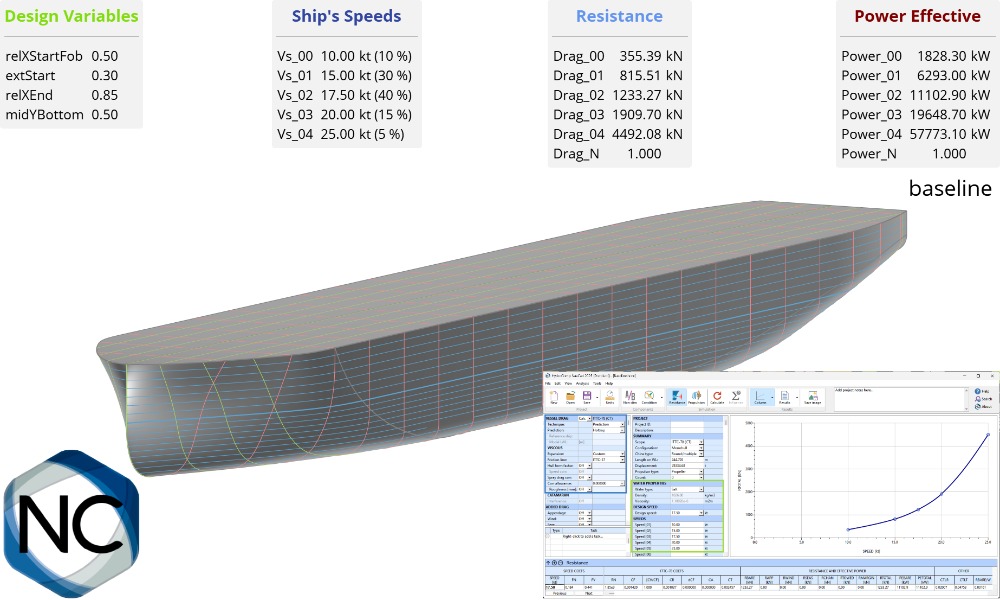
The NavCad connection with CAESES is enabled via the following CAESES feature definition:

• NavCad Bare Hull Resistance: Performs bare hull resistance calculations.

Click the button below to load the feature definition:

Load NavCad Connection Feature

Ship Hull Model

The ship model used in this tutorial is generated from the Ship Modeling Workflow. It is essentially the default parameterized model from the component-based ship, without a bulb or a skeg and with properties defined by the Ship Object in CAESES.

• Create a Component-based Ship from the Model workspace > Maritime tab > Ship > Component-based

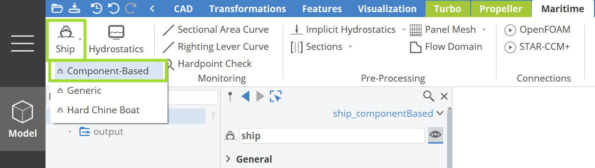
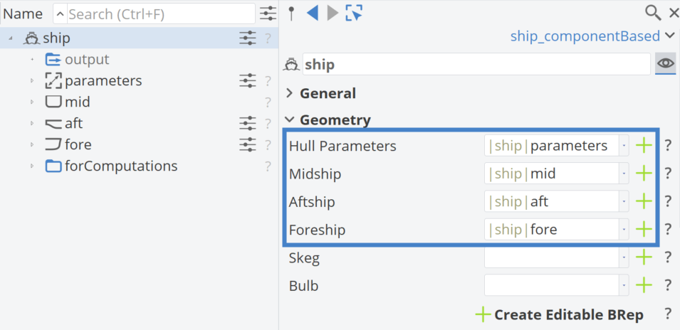
• Click the plus buttons in the Ship Object editor to add the:
  • Hull Parameters
  • Midship
  • Section-based Aftship
  • Waterline-based Foreship

This simple ship model will serve as a starting point for the NavCad connection.

NavCad Connection Overview

The NavCad connection is a two-step process: Configuration and Evaluation. In this setup, the bare-hull resistance of the vessel is calculated, along with the corresponding effective power. The purpose of this workflow is to first configure the NavCad project file and, once configured, proceed with the evaluation of the results.

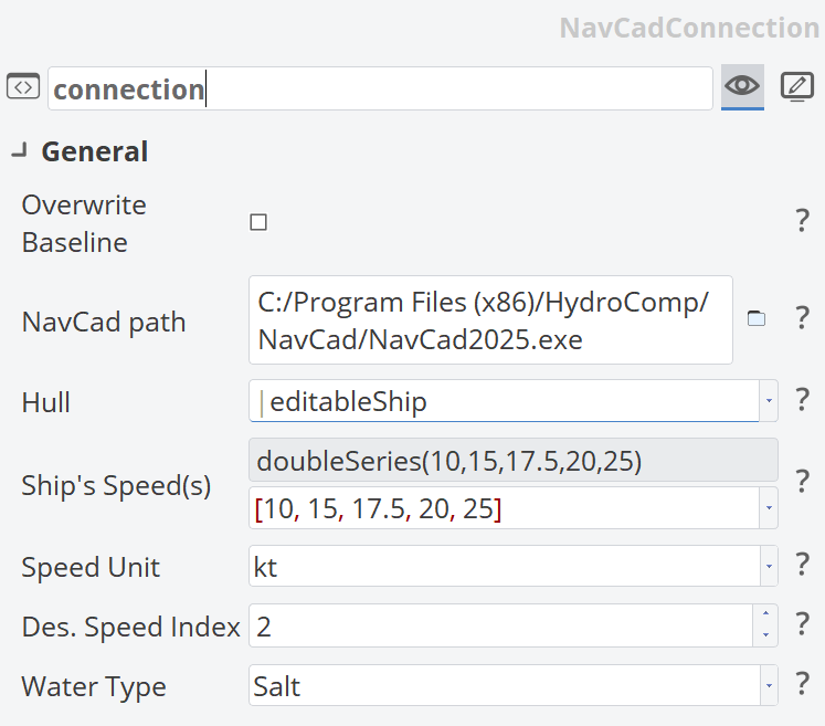
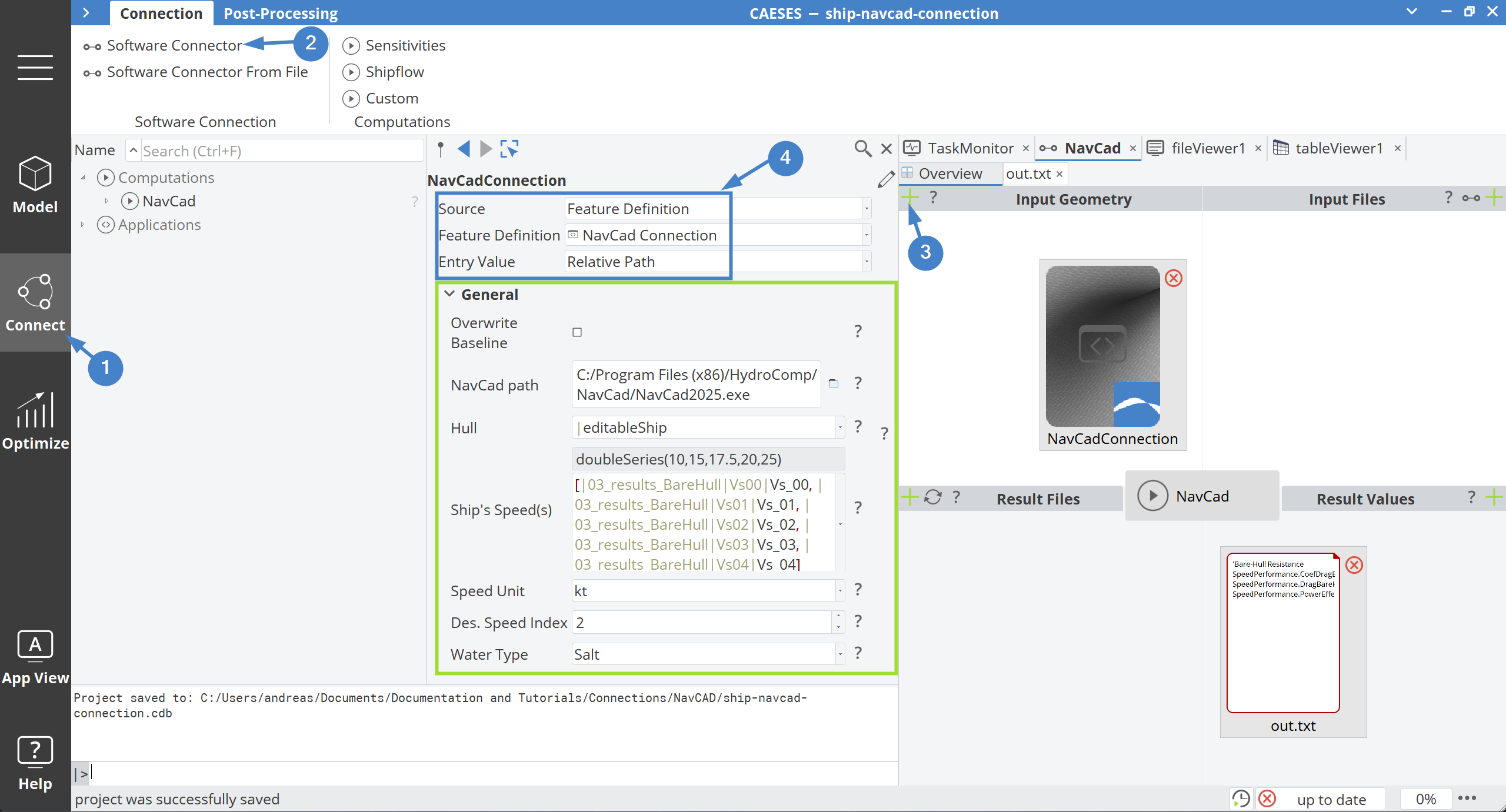
The figure below shows the required inputs to establish this connection:

• Overwrite Baseline (checkbox): When enabled, it re-runs the Configuration step.
• NavCad executable path: Typically located in Program Files (x86)/HydroComp/NavCad.
• Hull geometry: Either BRep or triangulated mesh. The hull must be properly floated according to the specified draft.
• Ship speeds: Defined as a Double Series.
• Speed unit: kt or m/s.
• Design speed index: For example, 0 corresponds to the first value in the Double Series.
• Water type: Select from Fresh, Salt, Brackish, or Custom.

To enable the connection:

1. Go to Connect in the Workspace Sidebar.
2. Create a new Software Connector.
3. Add the required Input Geometry.
4. Select Feature Definition as the source.

Results

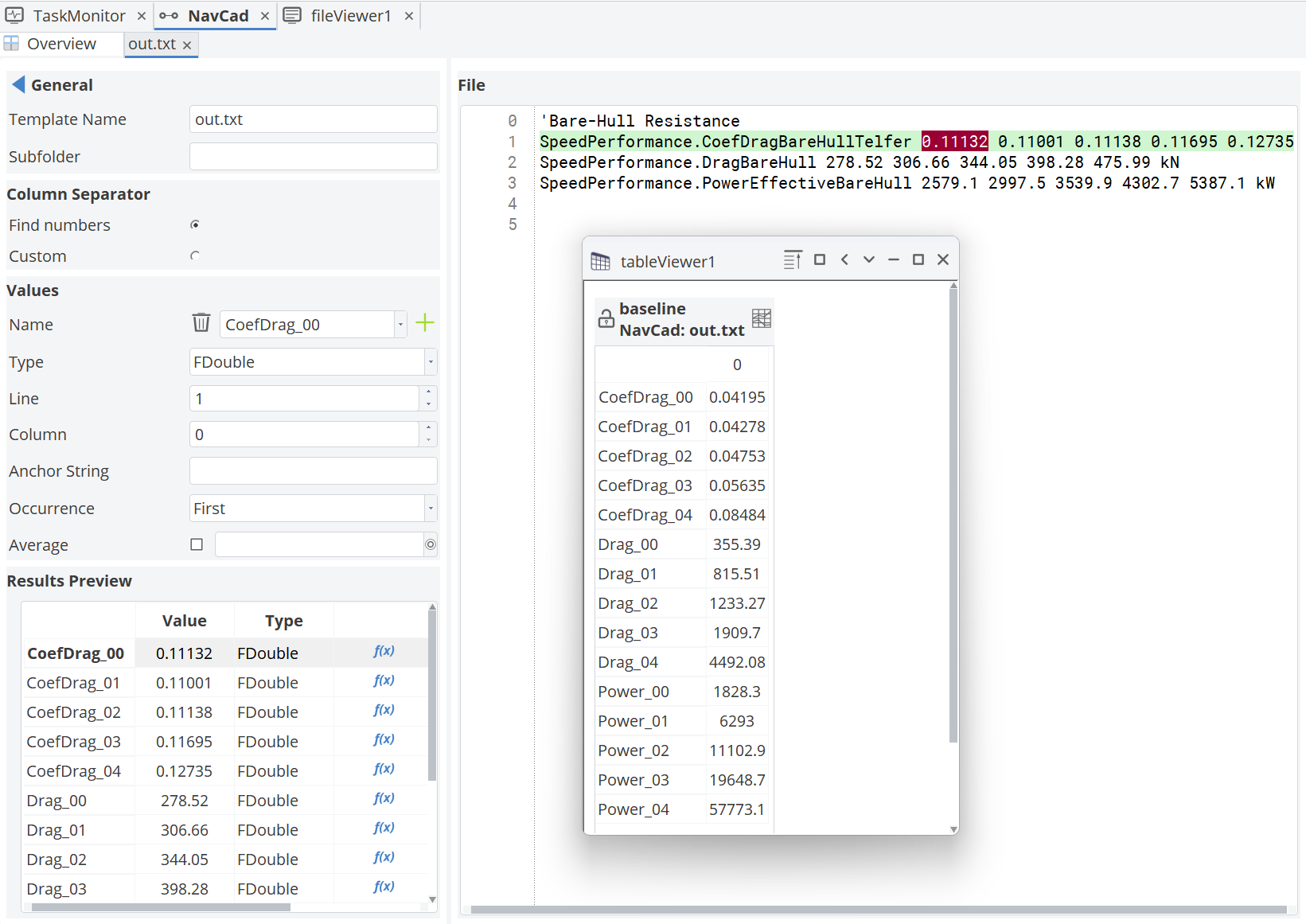
The NavCad connection produces result values in an out.txt file. For each defined speed, the following quantities are obtained:

• Bare-hull drag coefficient (Telfer)
• Bare-hull resistance (kN)
• Effective power (kW)

For example, if five speeds are defined, these three parameters are computed for each speed, as shown below.

Execution

To trigger the connection, an application must be defined in CAESES. A NavCAD_App is created, which executes the NavCadRun.bat script generated by the NavCad Connection feature.

Disable Asynchronous Update

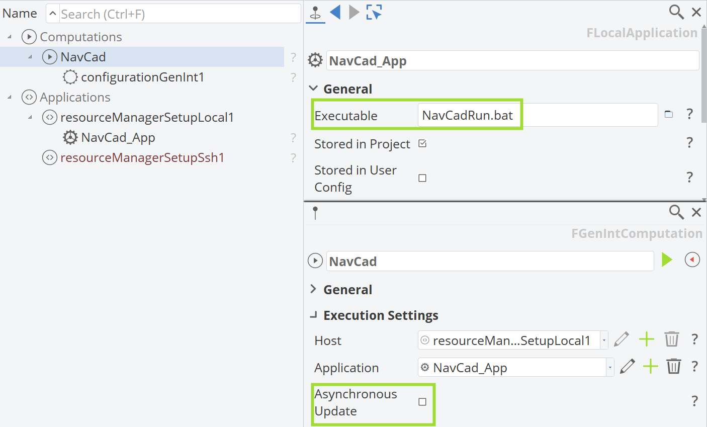
For the NavCad connection, it is important that Asynchronous Update is disabled (unchecked) to ensure robust operation.

Step One - Configuration

The first step of the connection launches the NavCad GUI. The purpose of this step is to allow the user to configure the NavCad project file, define analysis settings, and utilize hull variants from CAESES.

Within the NavCad interface, the vessel drag prediction method can be selected based on the design Froude number. Units, vessel speeds, and water properties are defined, along with environmental drag parameters such as wind and sea conditions. The ADVM (Advanced Viscous Model) method is typically selected for resistance prediction, with viscous expansion enabled.

Finally, the NavCad project file is saved as a calculation template for analyzing variants, typically named Baseline.hcnc.

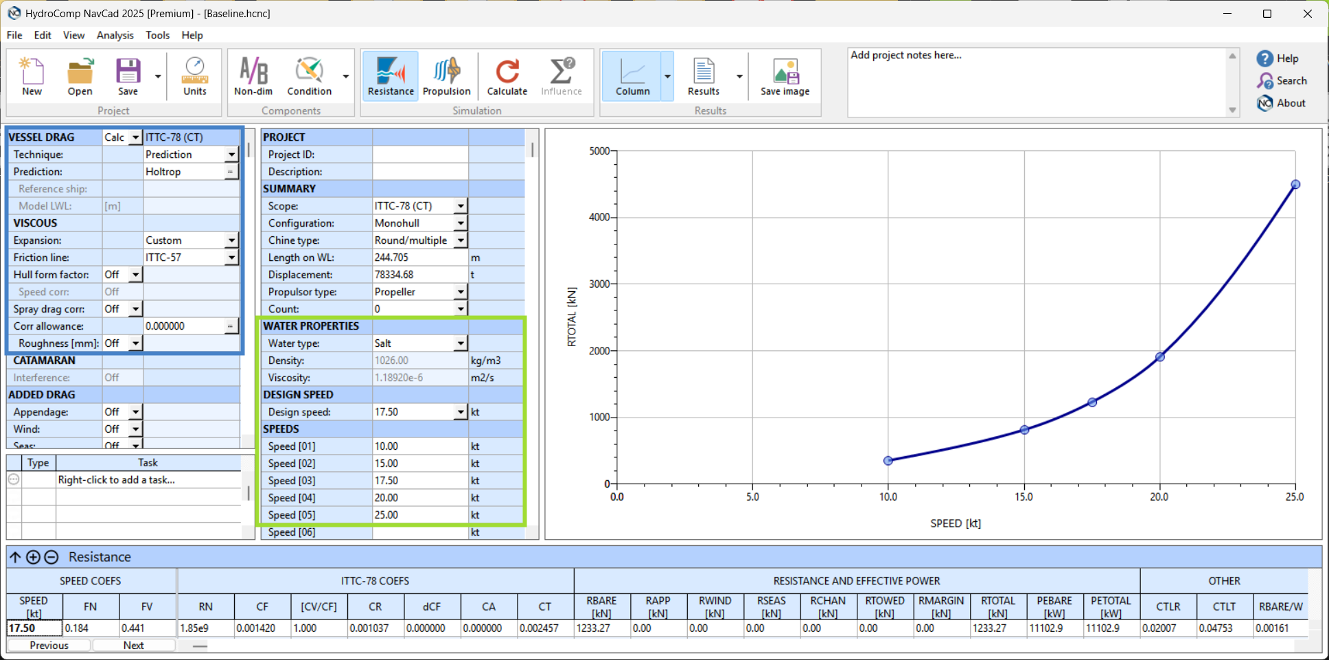
Behind the scenes, this step generates a Script.txt file containing commands that NavCad can interpret. This file is automatically created by the NavCad Connection feature.

selected prediction technique

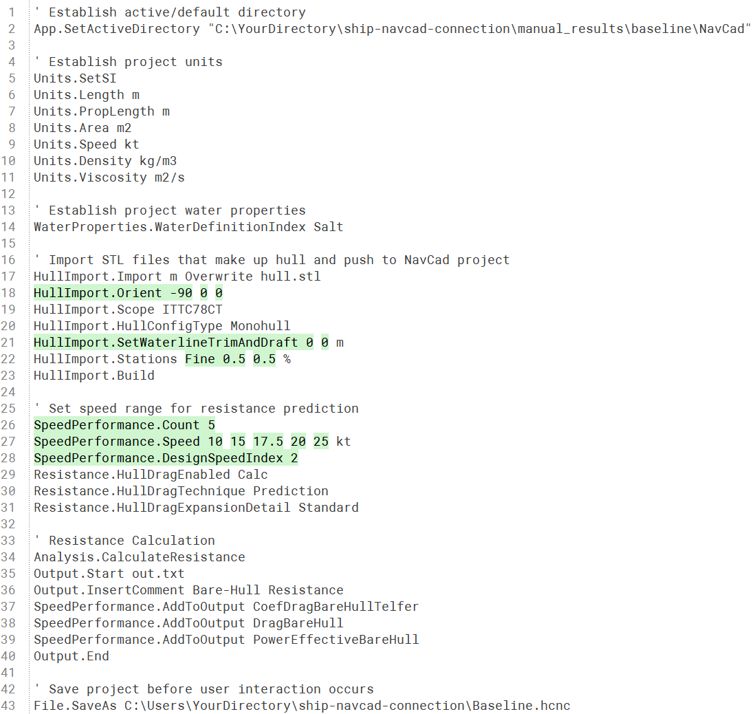
In this NavCad setup, the selected prediction technique is Holtrop, which is widely used and considered robust. For viscous resistance estimation, the ITTC-57 friction line is applied. These choices are well suited for the given Froude number range, although they can be adjusted if needed.

Step Two - Evaluation

Once the configuration is complete, the second step can be performed. This step evaluates the results based on the configured parameters, including the calculated resistance and effective power requirements.

Similar to the previous step, a different Script.txt file is generated, containing fewer commands, since the project has already been configured during the first step.

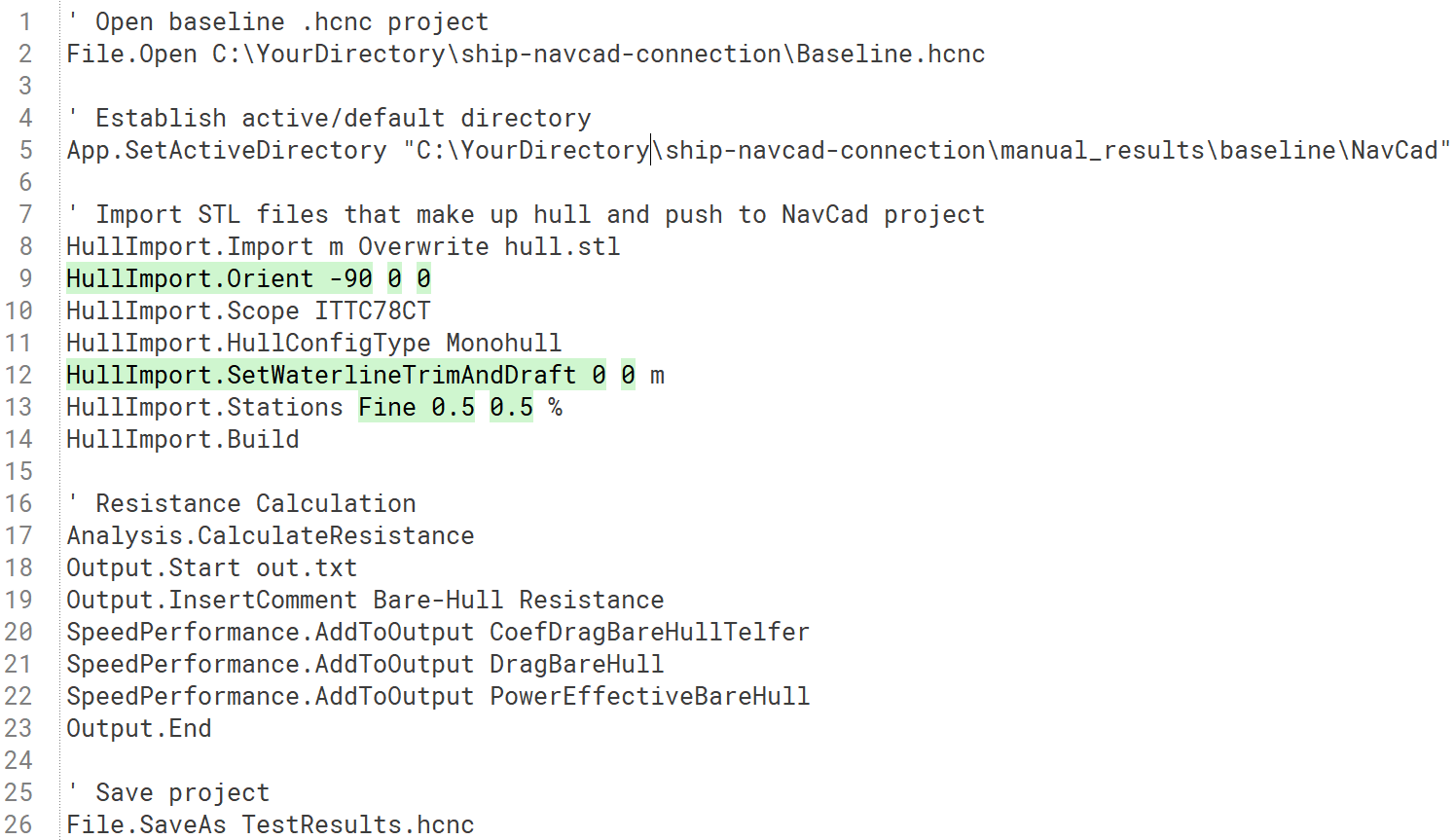
During the two-step connection process, a different executable, NavCad20xxRunScript.exe, is used instead of NavCad20xx.exe, which launches the NavCad GUI. In this step, NavCad runs in the background. You may notice the NavCad icon and a server process in the system tray handling the computations. This process is managed by the NavCad Connection feature.

info

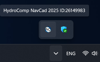
Running NavCad in the background enables a fully automated workflow that can be used for design space exploration or optimization processes. It is significantly faster than interacting with the GUI and avoids manual user input. For each design, a separate NavCad project file named TestResults.hcnc is created, which can be opened independently to review the results.

Design of Experiments (DoE)

The results generated in out.txt can be further utilized for design space exploration.

A Design of Experiments (DoE) using a Sobol sequence is proposed to monitor the effective power and bare-hull drag over a range of speeds. Since five different speeds are considered, a weighted average is used to compute a single representative value for performance.

For the speed range $V_i = [10,\ 15,\ 17.5,\ 20,\ 25]$ knots, the following weights $w_i$ (in percentages) are assigned:

$$w_i = [10\%,\ 30\%,\ 40\%,\ 15\%,\ 5\%]$$

The highest weight is assigned to the design speed at 17.5 knots.

Baseline Reference Values

The default parameters of the Ship Object are used as the baseline design. The corresponding reference values are:

Speed (kt)	Drag (kN)	Effective Power (kW)
10	355.39	1,828.3
15	815.51	6,293.0
17.5	1,233.27	11,102.9
20	1,909.70	19,648.7
25	4,492.08	57,773.1

note

Drag and effective power strongly depend on ship speed. Even when using weighted values, direct comparison may be misleading. Therefore, normalized parameters are introduced.

Monitored Parameters

The monitored parameters for the normalized effective power and drag are defined as:

$$P_{\text{norm}} = \sum_{i=1}^{n} w_i \cdot \frac{P_i}{P_{\text{ref},i}}$$ $$D_{\text{norm}} = \sum_{i=1}^{n} w_i \cdot \frac{D_i}{D_{\text{ref},i}}$$

Where:

• $P_i$ is the effective power at speed $V_i$
• $D_i$ is the drag at speed $V_i$
• $P_{\text{ref},i}$ is the reference effective power at speed $V_i$
• $D_{\text{ref},i}$ is the reference drag at speed $V_i$
• $P_{\text{norm}}$ is the normalized effective power
• $D_{\text{norm}}$ is the normalized drag
• $w_i$ is the weight assigned to speed $V_i$
• $n$ is the number of speeds

note

For the normalized parameters, a value of 1 corresponds to the baseline design.
Values < 1 indicate improved performance, while values > 1 indicate worse performance.

Design Space Exploration

This approach provides a single monitoring value for both effective power and drag, accounting for the relative importance of each speed.

In this example:

• Four design variables are varied:
  • Two for the aftship (relXStartFob and extStart)
  • Two for the foreship (relXEnd and midYBottom)
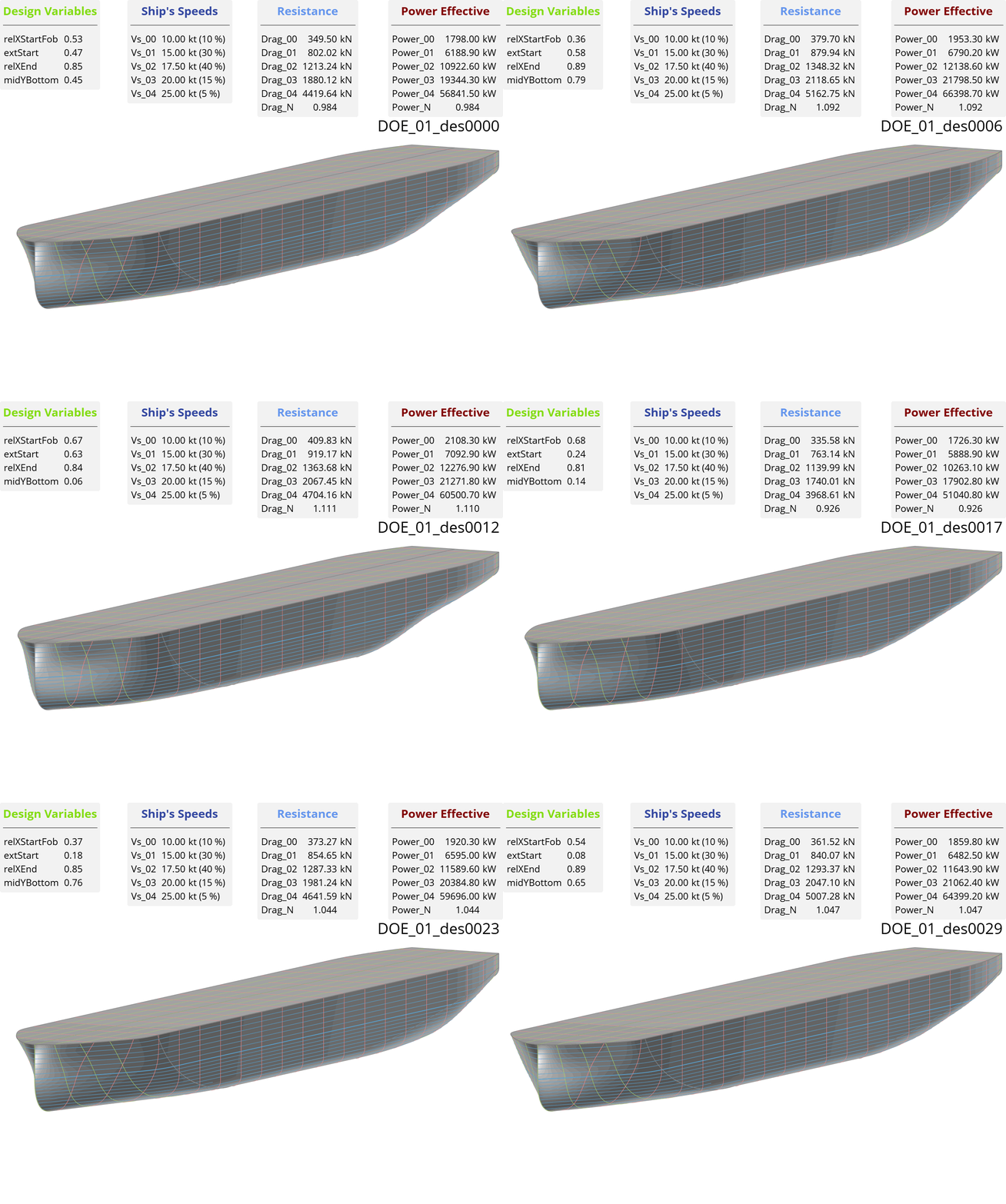
• A Sobol sequence with 30 design samples is used, which is sufficient to explore the design space efficiently.

The resulting variation in geometry and performance is illustrated in the animation below, where Drag_N and Power_N represent the normalized parameters.

Final Setup

CAESES Project File

If you want to take a look at the finalized software connection setup and the model you can find the resulting CAESES project file ship-navcad-connection.cdb here:

Download Final Setup

Disclaimer

We do not take any responsibility for the results obtained using NavCad or any of its components.