CFD Post-Processing

For Naval Architects and Marine Engineers

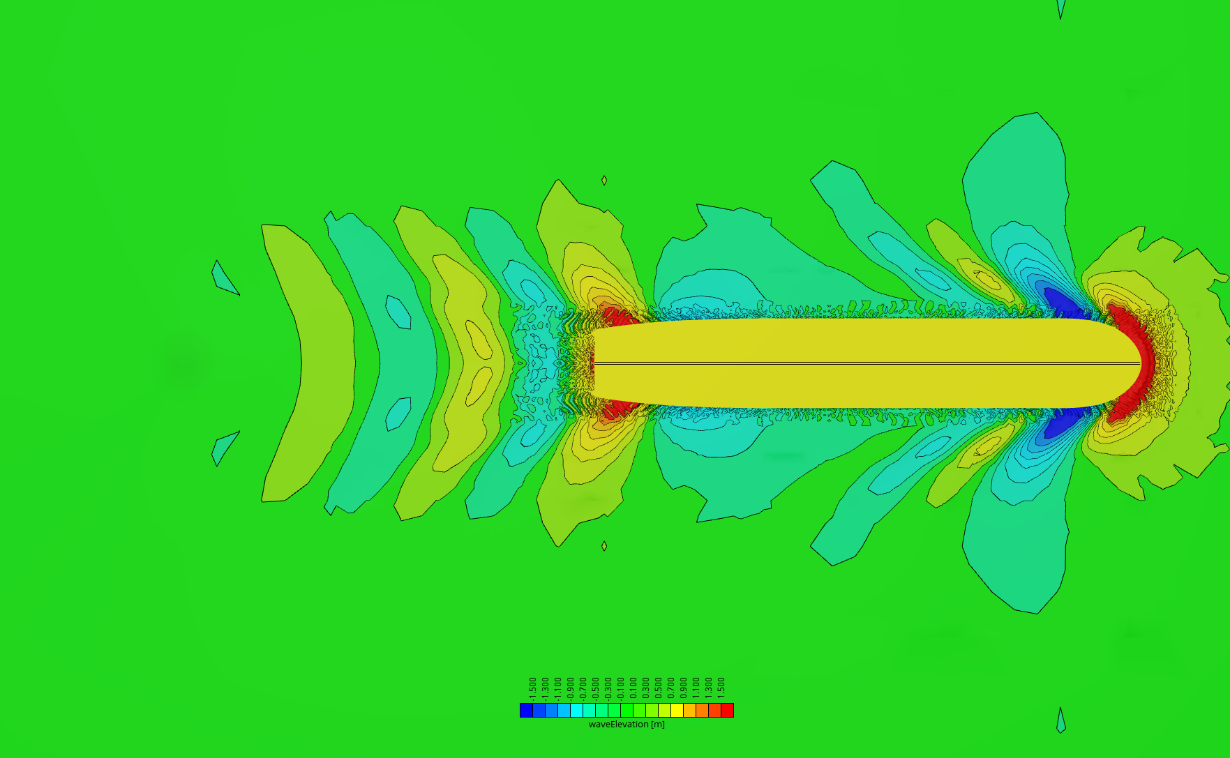
Viscous CFD-simulations - similar to model tests - are regularly carried out at model-scale to improve robustness of the simulation and reduce runtime. Obviously, as full-scale results are needed this required a model-to-full-scale transformation afterwards.

In this tutorial the setup of a Reynolds-transformation of integral values as well as preparation of visualizations is discussed.

It is assumed that time-series of forces and moments as well as VTK-files for hull and free surface, as resulting from the OpenFOAM-Connector tutorial, are available.The tutorial itself is based on these OpenFOAM® results, please modify as plausible for other CFD codes. Further, it is assumed that the user has some experience in using CAESES from the previous examples. Therefore not every step will be explained in full detail. Last, but not least, it is assumed that the user has a decent understanding of naval architectural model test and / or CFD procedure.

Nomenclature

Symbol	Meaning
$A$	Reference area [m²]
$c_{i}$	Coefficient of force $i$
$Fn$	Froude number
$g$	Gravity (usually 9.81 m/s²)
$L$	Reference length [m]
$R_{i}$	Resistance component $i$ [N]
$Rn$	Reynolds number
$U$	Speed [m/s]
$\nu$	Kinematic viscosity [m²/s]
$\rho$	Density [kg/m³]

Subscript	Meaning
$..._{M}$	Model (model-scale)
$..._S$	Ship (full-scale)

Integral Values and Reynolds-Transformation

The results files as generated by the CFD solver (or dedicated post-processing scripts for that matter), if configured appropriately in CAESES, can be found in Connect > Result Values and Result Files, respectively.

Time-Averaging of Integral Values

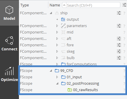
If not post-processed by other means (e.g. a dedicated script) the files in Result Values usually contain time series of integral values such as forces or moments. To use just the final number of interest would be simple but - in many cases - incorrect. Instead, if not post-processed by more involved methods like box-car averaging, these time series-have to be averaged over a meaningful number of time steps. To prepare the post-processing procedure first a new Sub-Scope "|99_CFD|02_postProcessing" is created in Model > CAD. Within this Scope a further Sub-Scope "|99_CFD|02_postProcessing|00_rawResults" is to be created and selected as Working Scope.

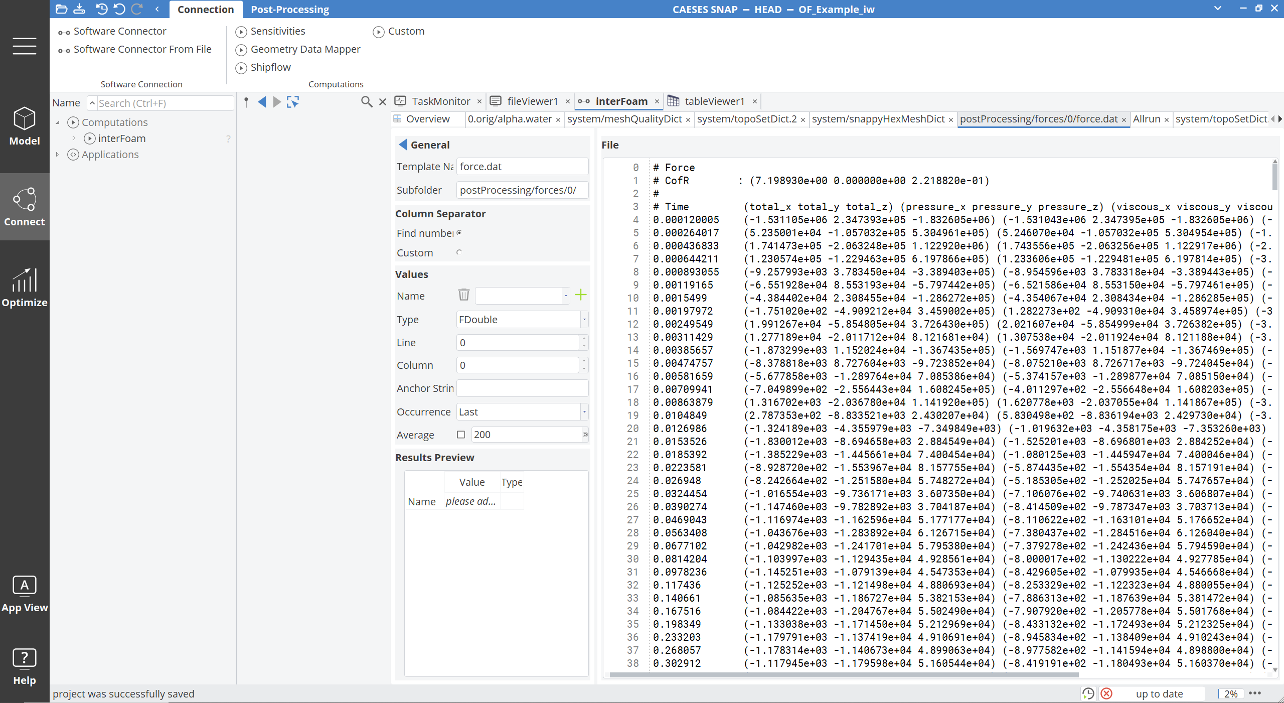
Next, in Connect > Result Values the File postProcessing/forces/0/forces.dat is selected:

To average the results and make them available in CAESES create a new Value Name ("Fx") in the General > Values Tab, select Average with a number of 200 and set Column to e.g. 1 for total_x. Repeat with FxP and FxV for Columns 4 and 7, respectively.

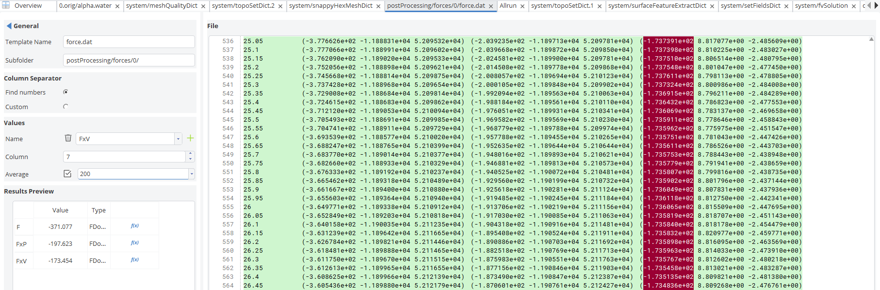
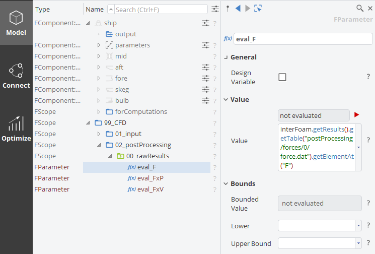
To make the time-averaged results available as Parameters hit the blue Parameter $f(x)$-button of each. Following this they will appear as Parameters eval_[...] in Model > CAD > |99_CFD|02_postProcessing|00_rawResults.

If not evaluated is shown as below, refresh by clicking Read existing result file in the Software Connector.

Model-to-Full-Scale Transformation

Keeping in mind that the forces evaluated above are values for only HALF a model, in model scale and model coordinate system, further post-processing is required. As described below for the Reynolds-transformation the further post-processing requires some a priori computation of additional data, namely the Reynolds-number at full and model-scale, the resulting friction coefficients and the wetted lengths and surface areas.

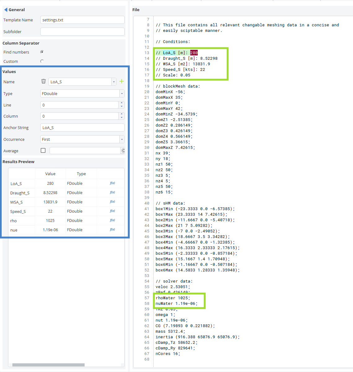
As the load case and operating conditions are selected in the Software Connector these values are extracted from the input file settings.txt generated by the Feature in the Software Connector for consistency. The required values can nicely be accessed by Anchor Strings, e.g LOA_S.

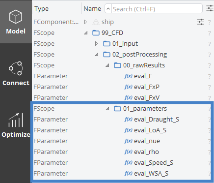
Extract the values as shown below and create parameters for further use in a Scope Model > CAD > |99_CFD|02_postProcessing|01_parameters:

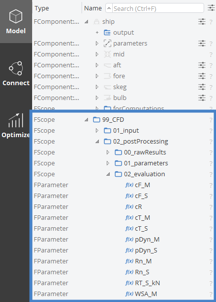
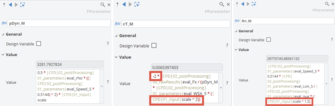
To execute the Reynolds-transformation the required information, as described in the explanation below, are computed as Parameters in Scope Model > CAD > |CFD|02_postProcessing|02_evaluation. In the following the computation of the Parameters will only be shown exemplarily.

caution

Please take care to use the correct scaling for length, areas, speed, ...!

In the end RT_S_kN will give the full-scale resistance (in kN if divided by 1000).

Reynolds-Transformation

To compute full-scale results from model tests or simulations carried out at scale it is essential that the tests or simulations have been carried out at Froude-similarity:

$Fn_{M} = Fn_{S}$ with $Fn=\frac{U}{(gL)^{0.5}}$

For the Reynolds-transformation it is assumed that the resistance of a ship (or a model thereof) can be decomposed in a friction and a residual component (or, coefficient based $c_{F}$ and $c_{R}$) with the frictional component computed according to the ITTC'57 friction line:

$c_{F}=\frac{0.075}{(log(Rn)-2)^2}$, with $Rn=\frac{U L}{\nu}$.

With coefficients in general being computed from forces by

$c_{i}=\frac{F_{i}}{0.5\rho U^2 A}$

it holds that the residual resistance coefficient $c_{R}$ is computed from the total resistance coefficient

$c_{T}=\frac{R_{T}}{0.5\rho U^2 A}$ by $c_{R}=c_{T} - c_{F}$.

Given Froude similarity (see above), it is assumed that $c_{R} = c_{RM} = c_{RS}$, whereas $c_{FM}$ and $c_{FS}$ are computed from $Rn_{M}$ and $Rn_{S}$, respectively. Contrary to the ITTC'78 procedure any form factor beyond that included in the ITTC'57 friction line is ignored and implicitly considered to be part of $c_{R}$.

Visualization

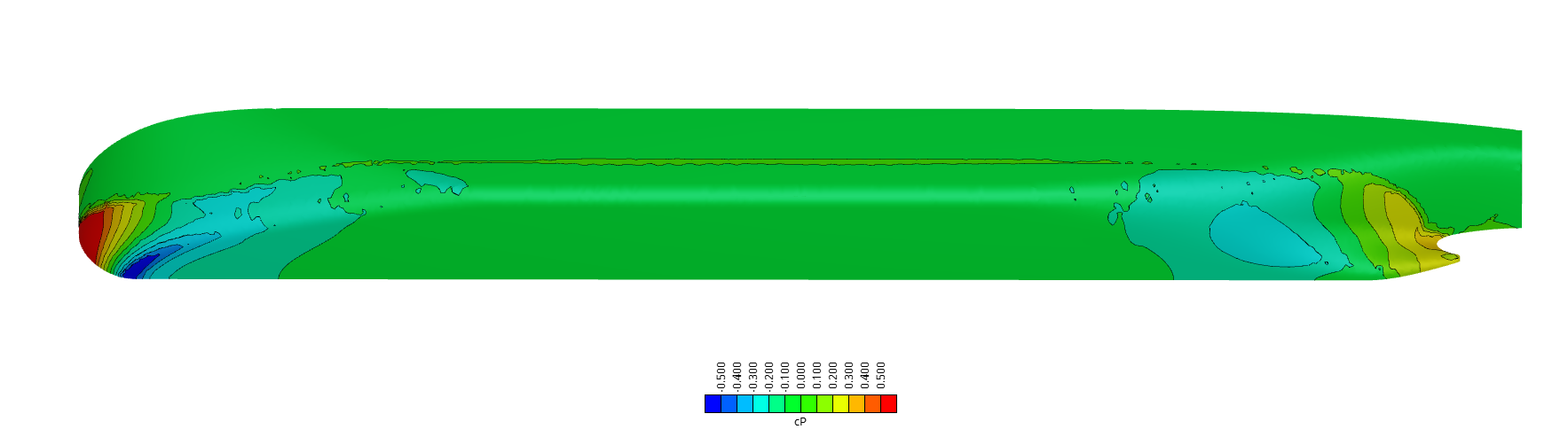
For the post-processing of CFD simulations it is common to visualize the pressure distribution by pressure coefficient ($c_{P}$) map and the free surface by a wave elevation map. As CFD codes usually provide the dynamic pressure, not $c_{P}$ and the free surface as geometry located at draught above Z-coordinate 0 on average (in model-scale!) these values have to be re-calculated for visualization.

It is assumed that the user is familiar with the generation of color maps in general, so only the specifics will be explained here.

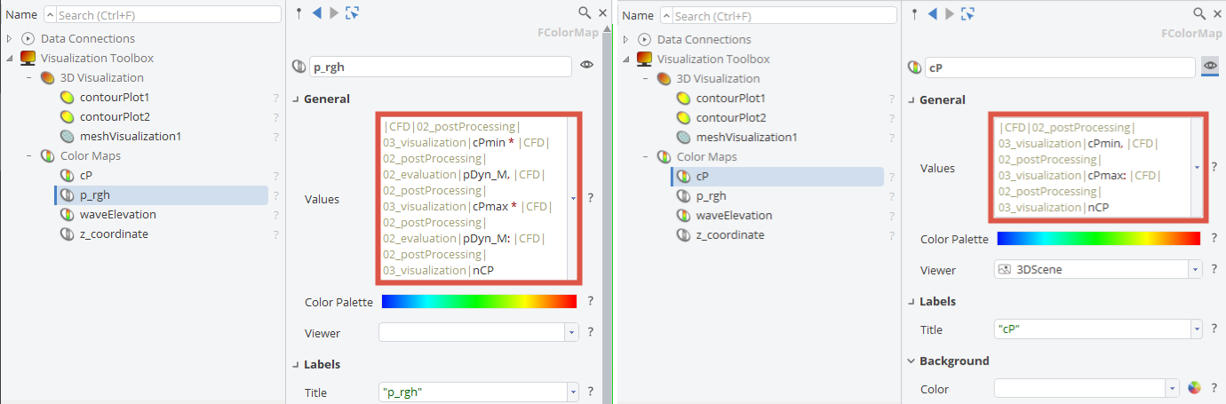
CAESES does not allow the further manipulation of results fields imported e.g. as VTK-files. Therefore the color maps have to be set accordingly with a minor work-around to show color legends for coefficients or wave elevation at full scale.

To this end scaling Parameters are created in the Scope Model > CAD > |99_CFD|03_visualization:

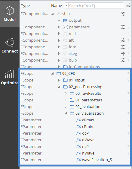
Parameter	Value
cPmax	0.5
cPmin	-0.5
dcP	0.1
ncP	$\frac{(cPmax - cPmin)}{dcP} +1$
waveElevation_S	1.5
dWave	0.2
nWave	$\frac{2 \cdot waveElevation_S}{dWave} +1$

To visualize e.g. the dynamic pressure field but scaled and annotated as coefficients first a Contour Plot of said field has to be created in Connect > Post-Processing:

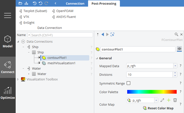
The key for the intended visualization by $c_{P}$ is to create Color Maps for p_rgh and $c_{P}$ set to ranges connected by the parameters defined in Model > CAD > |99_CFD|03_visualization.

tip

Take a look at the CFD results comparison tutorial to learn more about the results comparison functionalities in CAESES.