Curves

CAESES provides a set of different parametric curves c(t) that can be found in the menu

• Model > CAD > Curves.

This section gives you a brief introduction the most important curve know-how. Check the help-icons, a question mark icon (?), of the properties to learn about each individual input of the different curves.

In CAESES, NURBS (Non-Uniform Rational B-Splines) are employed to represent and manipulate complex geometric shapes. For detailed information check the NURBS Explained section.

Curve Types

The different curve types are grouped by the inputs to create the curve. These are:

• Point Based
• Curve Based
• Surface Based
• BRep Based

FCurve

This curve is the basic type for curves. Every other curve type is in the hierarchy below the FCurve. The functionality of this curve is to provide a Creation Method, which can be dynamically switched, which also gives it the name "Dynamic Type".

tip

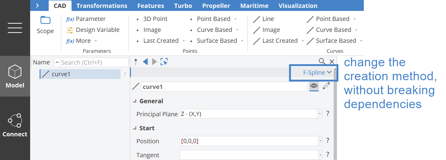
When the Creation Method is changed, all dependencies to this curve will be preserved.

Apart from standard B-Spline and NURBS curves, some of the most important alternatives are:

• F-Spline: A curve with additional control over tangents and curvature at the start and end, as well as, the control centroid and the curve’s enclosed area.
• Interpolation: Generates a curve that passes exactly through a given set of points by selecting different interpolation methods.
• C-Spline: Approximates a set of points using a least-squares approach. The degree of the internal B-Spline curve as well as the number of control vertices can be specified.

Curve Properties

Curve Parameter T

The curve parameter "t" always runs in the interval [0,1], and can be used e.g. for calculating curve quantities such as position or tangent angles at specific curve locations.

FCurve

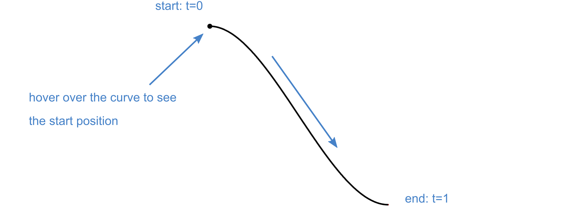
No matter which curve you consider (line, circle, NURBS etc.): All of these types have the same parent type FCurve, which provides the base functionality such as the command .getPos(), see the section "Curve Positions" below.

Start and End Positions

For a curve with the name "c", the start and end position can be received through the commands:

c:start

c:end

Note that these two properties return vectors (e.g. [1,2,3]).

tip

When you hover over a curve with the mouse cursor or if you select a curve, the start position is indicated by a small circle in the 3D view.

Curve Positions

In order to calculate and receive a curve position, use the position command:

c.getPos(t)

where t can be a value in the range [0,1]. This returns a vector.

Point positioned on curve

When you select a curve and create a 3D point (while still having the curve selected), it will automatically create the point on the curve using the position command.

Curve Creation

Typically, you create a curve and then set the properties. For instance, you create a line and then drag & drop the start and end position into the object editor (of the selected line object).

Create from a Selection

You can also take into account a selection. Most of the curve types come with a convenient creation mechanism that allows you to create a curve that takes into account the current selection. For instance, if you select two points and then create a line, the two points will be automatically set as start and end position. Such a mechanism is also helpful for splines and interpolation curves, for instance.

Display Options

Curves have a set of display options which are useful during modeling. Examples are the color, size (displayed thickness), curve points parametrization (to understand the parametric domain), curvature visualization or stipple pattern. Not all these options are shown in the user interface by default - just click on the display options category to expand 2nd level options.

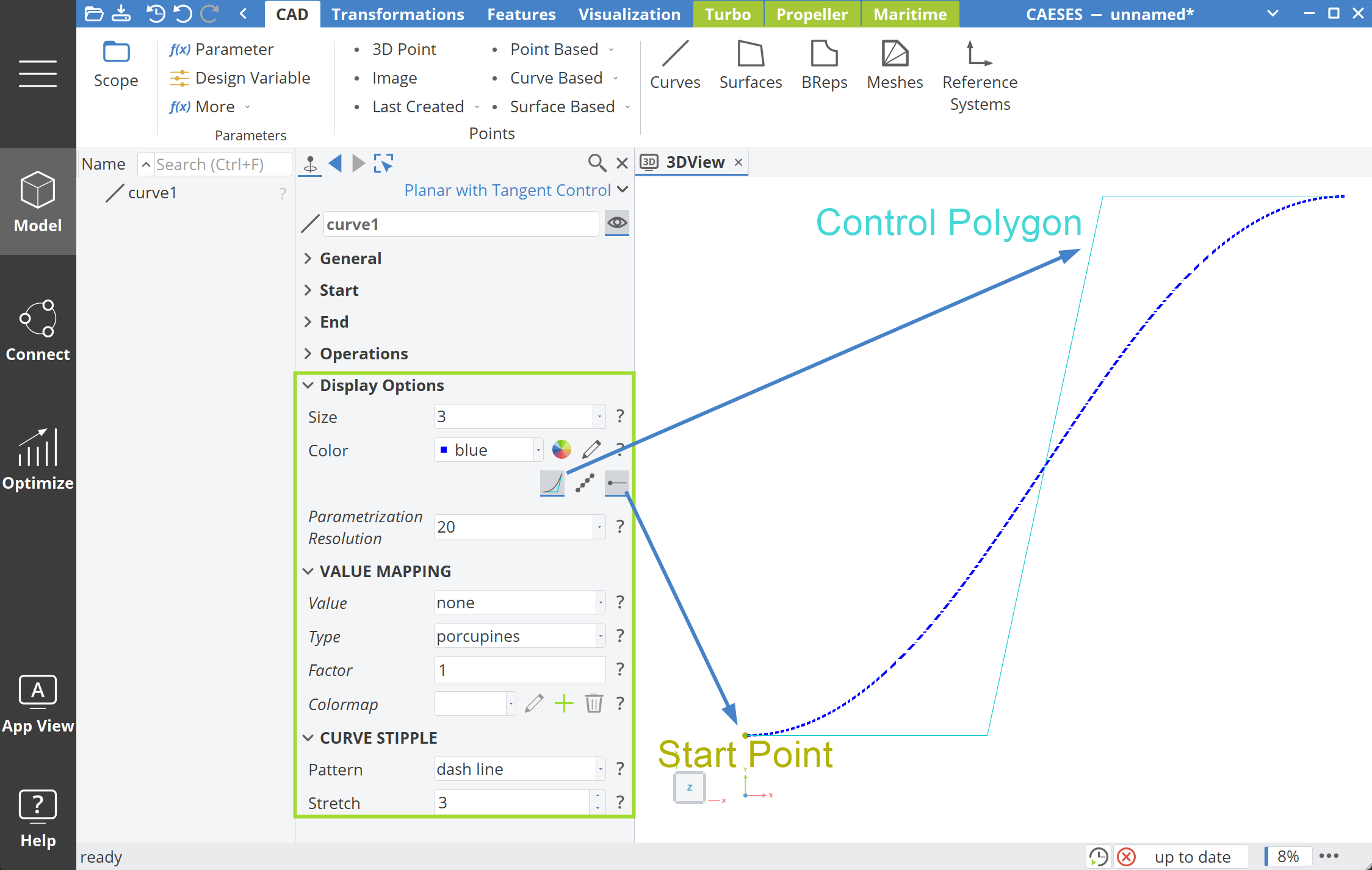
These display options can be toggled by clicking on the icons:

• Control Polygon: Shows the straight line connecting the control points (in light blue). While the NURBS curve doesn’t necessarily pass through all control points, the control polygon provides insight into the general direction and shape.
• Parameterization: Displays points along the curve at equal distances in the parametric domain [0,1].
  • Parameterization Resolution: Sets the number of points used to visualize the parameterization.
• Origin of the Curve: Marks the curve’s starting point.

Value Mapping on Curves

This option allows mapping scalar values along the curve for visualization.

• Value:

  • Curvature: Visualizes the curvature of the curve (rate of change of tangent direction).
  • Torsion: Visualizes the torsion of the curve (rate of change of curvature, twisting out of plane).

• Type: visualization styles for mapped values:

  • Colored line
  • Porcupines (normal/tangent indicators)
  • Colored circles
  • Colored tube

• Factor: Scaling factor applied to the mapped values.

• Colormap: Defines the color scheme for mapping (default is usually sufficient).

Curve Operations

You can add post-processing operations in the Object Editor of the curve to further process it. It is an easy way to e.g. trim the curve, translate or rotate it, edit the control polygon or extend the curve. Check the type documentation for details on each operation.

Access Output from Operations

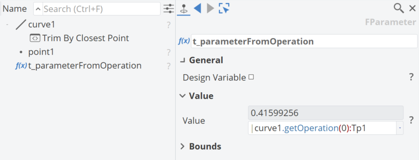
You can access the output from feature-based post-processing operations by using the command .getOperation(Index).

In the example a curve is trimmed by the closest point. In order to access the t parameter position of the trimming location you could create a parameter with curve1.getOperation(0):Tp1.

Edit Curve Control Polygon

For each curve in CAESES (which is generally represented internally by a NURBS formulation), in the Object Editor in the category Operations you can find the option Edit Control Polygon.

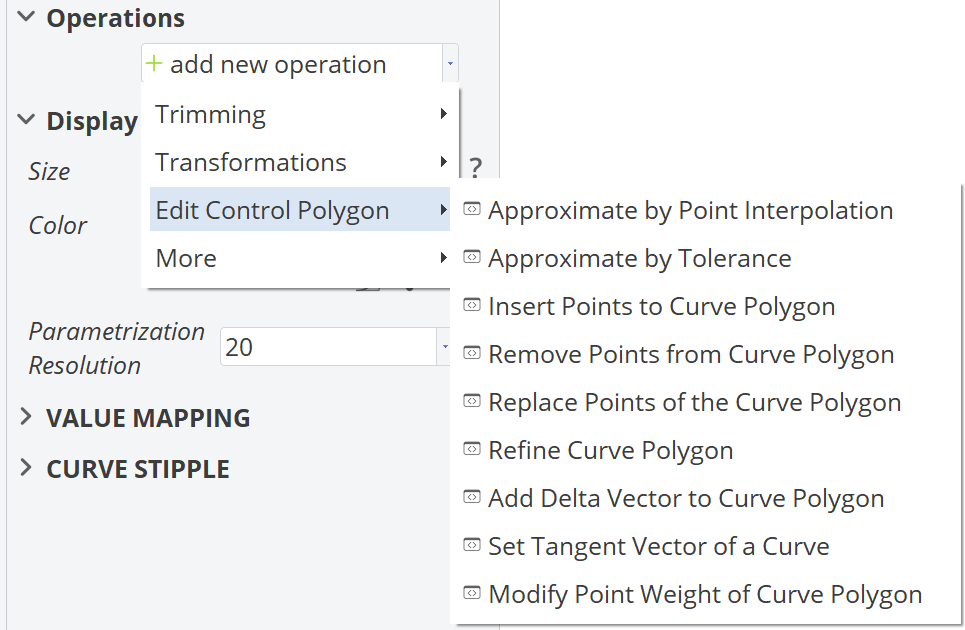
• Approximate by Point Interpolation: Approximate the curve by interpolating given points.
• Approximate by Tolerance: Approximate the curve within a specified tolerance.
• Insert Points to Curve Polygon: Add new control points to the polygon.
• Remove Points from Curve Polygon: Delete selected control points.
• Replace Points of the Curve Polygon: Substitute existing control points with new ones.
• Refine Curve Polygon: Add refinement points for higher accuracy.
• Add Delta Vector to Curve Polygon: Adjust control points by applying a vector offset.
• Set Tangent Vector of a Curve: Define a tangent direction at the start or end of the curve.
• Modify Point Weight of Curve Polygon: Change the weight of a control point to influence the curve shape.

Enable the curve's control polygon to inspect the changes and make them visible in the 3D view.

Curve Parameterization

The parameterization of a curve defines how its parameter space is distributed along its length.
This is particularly important when the curve is used as input for surface generation, since the parameterization can affect the resulting surface shape.

In CAESES, there are two main categories of parameterization options:

• Automatic (no input required): a parameterization method is applied directly.
• Manual (input required): additional input (e.g. reference curves, weights, scaling factors) is required along with the chosen method.

normalized arc length

To better understand the parameterization options in CAESES, it is important to clarify that the function $s(t)$ represents a normalized arc length parameter, defined over the interval [0,1].

Automatic Parameterization Options

info

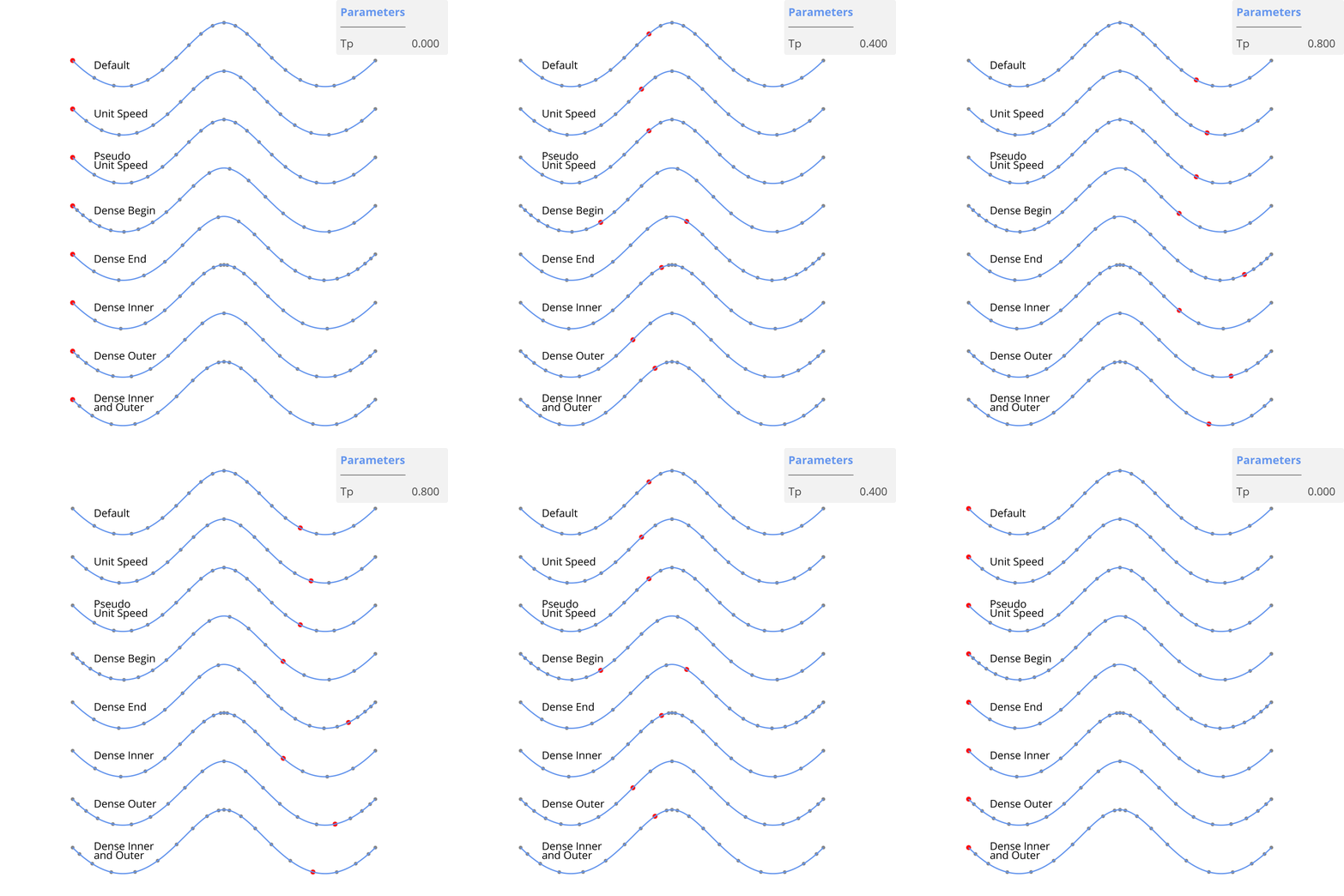
The parameter Tp shown in the animation corresponds to the curve parameter t, which always varies within the interval [0,1].

Default

The curve keeps its natural parameterization, with no re-approximation or modification.

Unit Speed

The parameterization is set to: $s(t) = t$

This means that the curve parameter t changes uniformly with respect to the curve’s arc length.

Dense Regions (Outer / Begin / End / Inner / Inner and Outer)

Uses predefined parameterization functions so that the derivative (or “speed”) $\frac{ds}{dt}$ is lower in the specified regions, resulting in denser point distribution there.

Pseudo Unit Speed

Produces a parameterization similar to the curve’s natural parameterization by scaling the knot vector accordingly, without approximation. This option also works if the given default parameterization is discontinuous (e.g., in Polycurves).

Manual Parameterization Options

Custom: $s(t)$

Allows specifying a custom parameterization function $s(t)$ in the x–y plane over the interval $x, y \in [0,1]$,
where the y-axis represents the mapped parameter, i.e. $y(x) = t_{\text{new}}$.

The function must be strictly monotonic, meaning that $t_{\text{new}}$ increases continuously from 0 to 1.

Mapped: $s(t)$

Uses a parameterization function $s(t)$ extracted from another curve. This allows reusing a reference curve so that the new curve inherits the same parameter distribution.

Mapped: $x(t)$, $y(t)$, $z(t)$

Allows reusing the parameterization of a reference curve based on individual coordinate mappings. The new curve inherits the same $x(t)$, $y(t)$, or $z(t)$ distribution from the reference curve.

tip

When using Mapped: $x(t)$ / $y(t)$ / $z(t)$ parameterization, it is recommended to select a reference curve that is monotonic in the corresponding direction (x, y, or z).
This ensures that the mapping remains valid and avoids ambiguous parameter associations.

Mapped Parametrization Options

It is important that both curves share the same interval with respect to the selected direction.

Otherwise, zero- or infinite-speed regions may occur near the curve ends, which can lead to downstream problems.

Mapped: Shortest Distance

Defines a parameterization function derived from a reference curve, aligning corresponding x, y, and z positions between both curves for equal values of t.

Shortest Distance

When using Shortest Distance parameterization, be cautious — multiple points on the target curve may have the same shortest distance to the reference curve. This can lead to singularities or abrupt parameter jumps.

Mapped: Shortest Distance (Smooth)

Uses a parameterization function $s(t)$ that mimics a true shortest distance mapping while avoiding singularities or ambiguities. This method is particularly robust for constructing Ruled Surfaces, Meta Surfaces, Lofted Surfaces, and similar curve-based geometries.

Shortest Distance (Smooth)

When using Shortest Distance (Smooth) parameterization, it is recommended to set the reference curve to Unit Speed or Pseudo Unit Speed for consistent spacing.

You can also adjust the Smoothing parameter, which is the maximum number of shortest distance pairs between curves. A value in the range of 5 to 15 is typically a good compromise between smoothness and accuracy (default = 10). The minimum allowed value is 4. If a lower value is specified or the smoothing does not succeed, the parameterization will fall back to the Default Parameterization.

• Increase the Smoothing parameter to obtain smoother transitions with fewer control points.
• Decrease the Smoothing parameter to capture more local detail with a denser parameter distribution.

Change Parameterization

change parameterization

Changing the parameterization can be helpful in very specific situations. However, it is recommended not to change this if not really required. Internally a new curve needs to be generated that is only an approximation of the original curve. This might cause problems in some solid modeling operations with BReps.

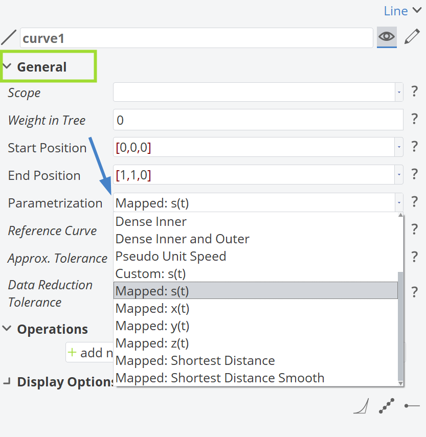
To apply or modify a parameterization for a Curve in CAESES, you can do this in two ways:

Option 1 – Under the General Label

Unfold the General label in the Object Editor to access parameterization settings.

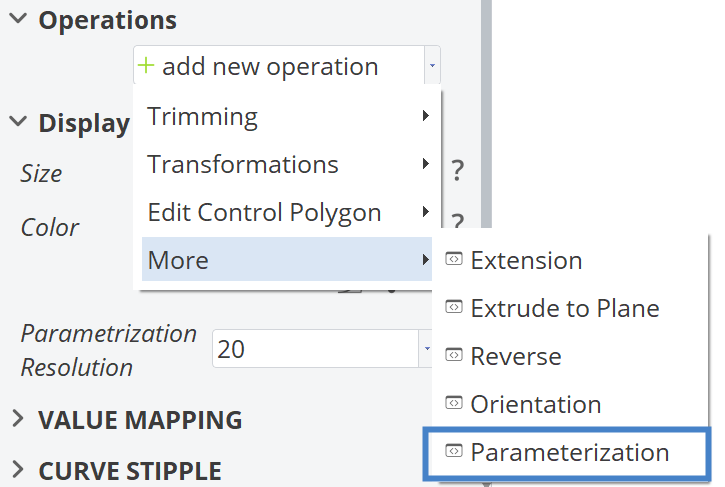
Option 2 – From Operations

In the Object Editor of the curve navigate to Operations → More → Parameterization.

Useful Commands

Below are some useful commands in CAESES that help analyze and work with curve parameterization.

• getPos(t)
  Returns the position vector of the curve at a given parameter value t in [0,1].
  The returned vector can be queried using .getX(), .getY(), and .getZ().

• getPosAtArcLength(const FDouble arc_length)
  Returns the position vector at a given relative arc length along the curve.
  The arc length is specified in normalized form in the range [0,1].

• getParameterAtArcLength(const FDouble arc_length)
  Returns the curve parameter t corresponding to a given relative arc length.
  This is useful for converting from physical distance along the curve back to parameter space.

• getLength(const FUnsigned resolution = 100)
  Computes the discrete length of the curve using a specified sampling resolution.
  Higher resolution values increase accuracy at the cost of computation time.

• getLengthFromTo(const FDouble from, const FDouble to, const FUnsigned resolution = 100)
  Computes the discrete length of the curve within a specified parameter range t $\in$ [from, to].

Tips and Tricks

Smooth Transitions

In order to create a smooth transition in 2D from a location A to a location B, you can use the F-Spline curve. It allows you to set the tangent angles at location A and B, and creates a fairness-optimized spline. You can find it in the menu

• Model > CAD > Curves > Point Based > F-Spline.

The F-Spline gives you additional area control so that you can set an integral area that is taken into account during curve creation. This is useful for controlling cross-section areas of profiles, airfoils and ship hull sections, for instance. There are more options available for the F-Spline, such as the centroid setting and curvature controls.

caution

Make sure to set the correct principal plane (property of the F-Spline) if you use this curve type. Otherwise the angle settings are not correct and the spline generation will not work.

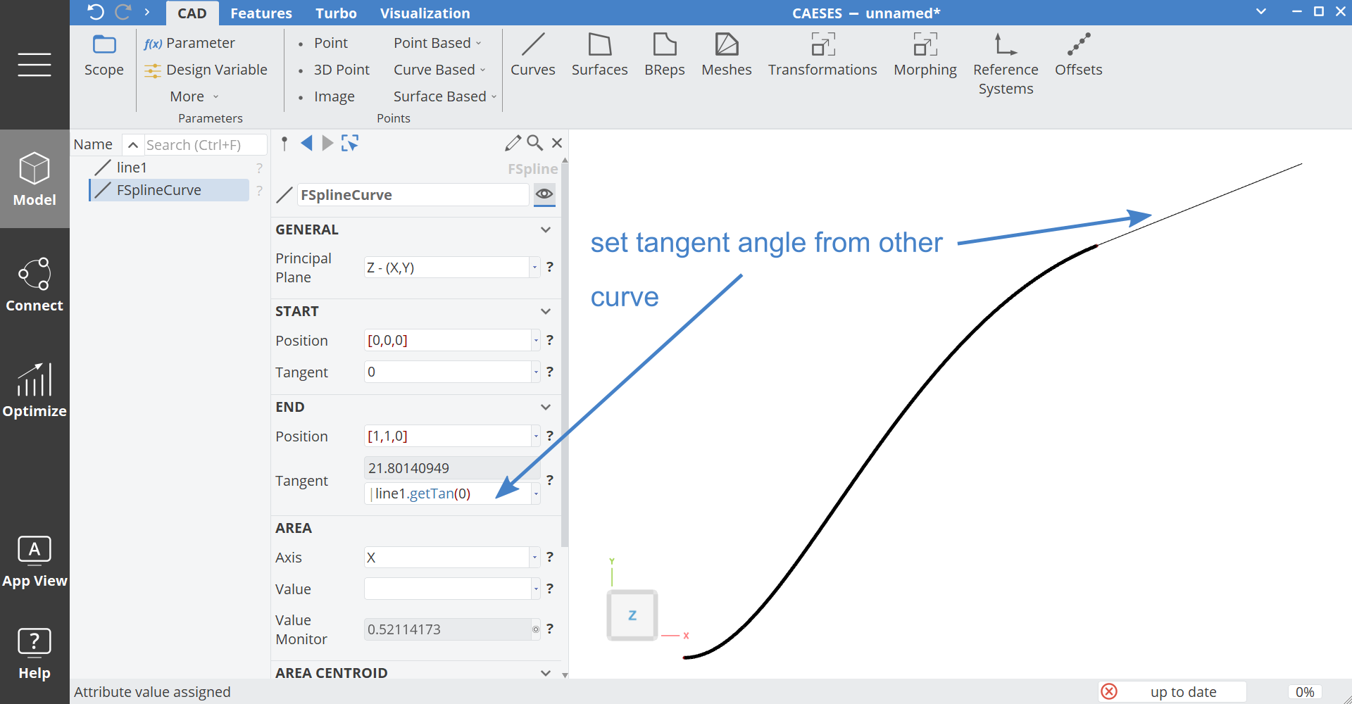
The so-called fillet curve allows you to create a smooth transition in 2D and 3D, but with less control.

Approximation

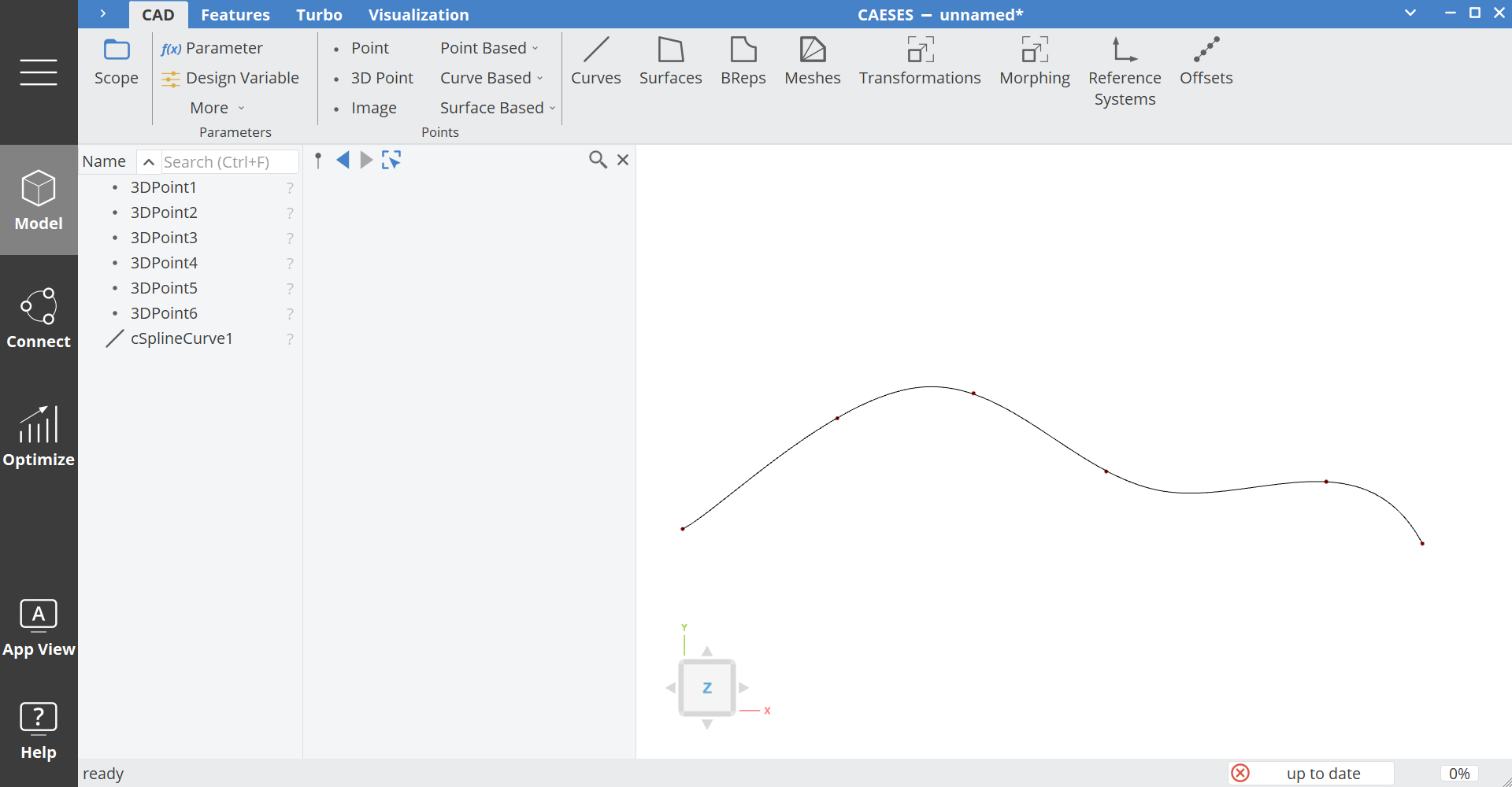
The C-Spline curve creates a smooth curve on the basis of a given point set. Typically, the points are not interpolated. There is a regression strategy applied (least-square) to create the curve. You can find it in the menu

• Model > CAD > Curves > Point Based > C-Spline.

Interpolation

Choose the interpolation curve in order to interpolate a set of points. You can find it in the menu

• Model > CAD > Curves > Point Based > Interpolation.

If you need to control the tangent angles at the given point locations, enter the following expression (pair: [point, tangent angle]) into the point list: [p1,0].

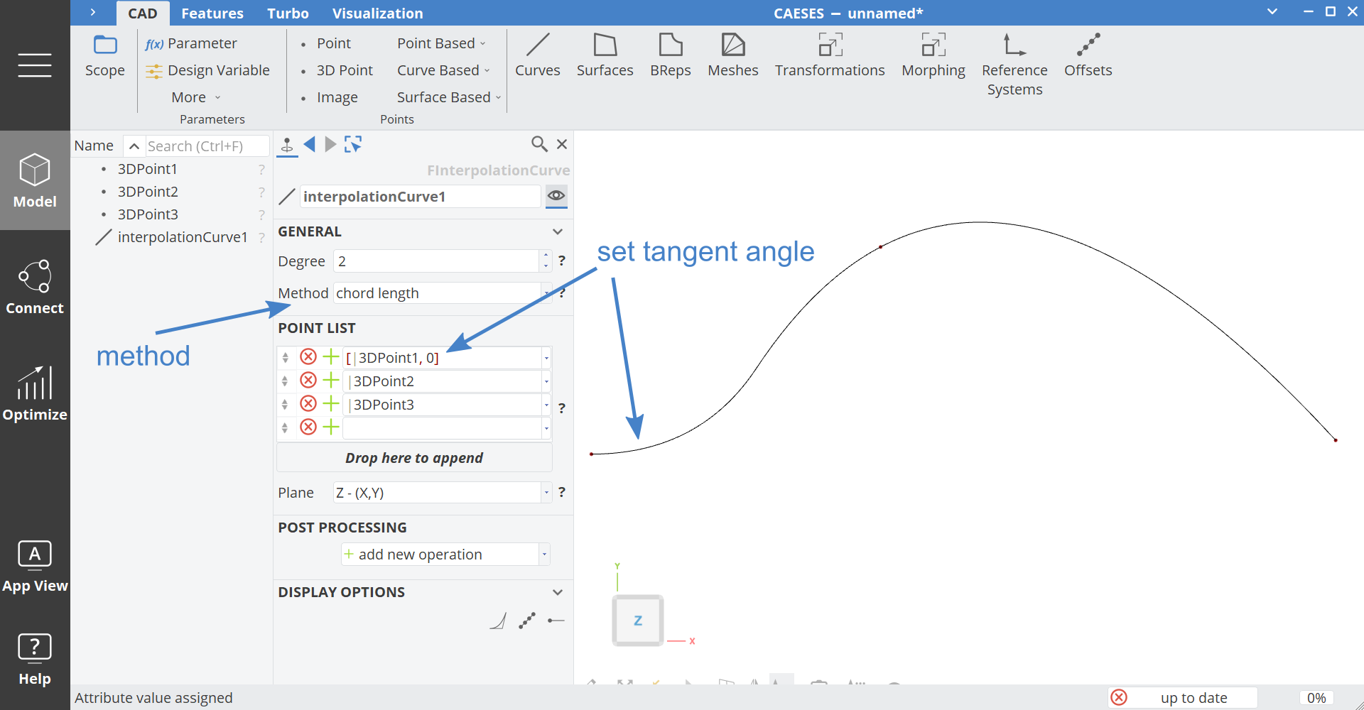
This would result in a tangent angle setting of 0 degrees at input point p1 of the curve. This helps to control peak points (zero tangent angle) or start and end angles of the interpolation curve.

If you choose the method uniform, centripetal or chord length at the interpolation curve, you can use additional options.

Instead of angle values, you can also enter a vector to define the curve tangents at the start and end position (i.e. for the first and last point of your input data). Here is an example:

[p1,[1,1,0]]

Here are examples with expressions, e.g. to take the vector information from another curve or surface:

[p1,curve.getTanVec(0.5)]

[p1,surface.getDU(0.5,0.5)]

Reversing Curves and Subcurves

You can use the image curve to reverse any curve (set the domain from [0,1] to [1,0]) or to create a subcurve by changing the domain (e.g. [0.25,1]). You can find it in the menu

• Model > CAD > Curves > Curve Based > Image Curve.

For instance, you can use the command .ft(0,0.25) to get the t position at an X-value of 0.25:

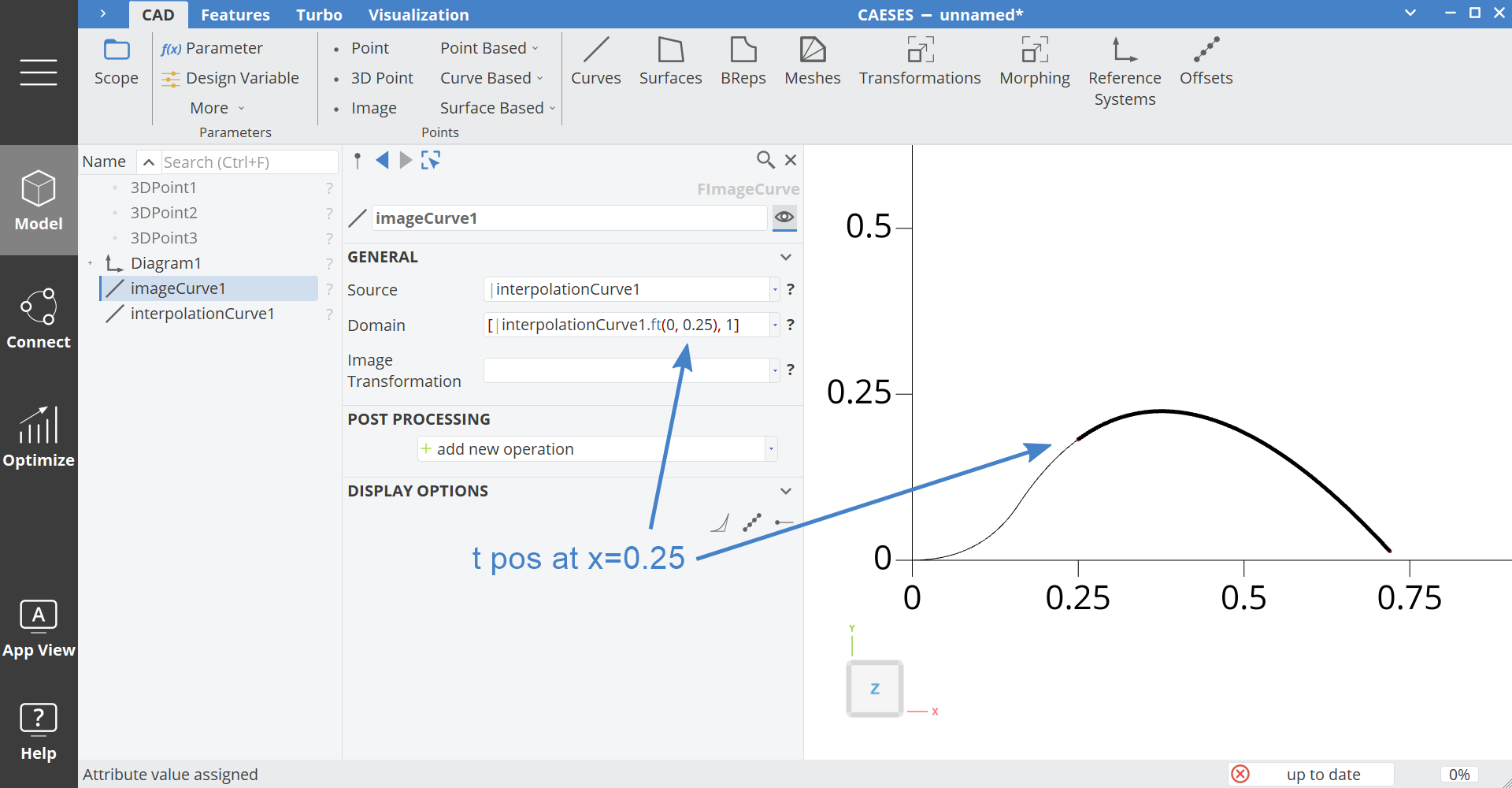
.ft

The command .ft() calculates the intersection position parameter t of the curve with respect to a given abscissa axis and elevation (and an optional parameter range).

The first input argument defines the axis:

• the X axis corresponds to the index: 0
• the Y axis corresponds to the index: 1
• the Z axis corresponds to the index: 2

In this example we are searching for the curve position parameter value along the X axis (0) at the elevation of 0.25.

Extrapolation

Extrapolation can also be done through the imagecurve: Just set the domain to e.g. [-0.1,1.1] to extrapolate the curve at the start and end location.

Offset and Section Modeling

The offset curve is a key type when it comes to profile and section modeling for blades and wings. You can find it in the menu

• Model > CAD > Curves > Curve Based > Offset Curve.

It allows you to set a thickness distribution that can be applied to a source curve (camber). The offset curve also has a constant offset option, to use a single value for offsetting a source curve.

info

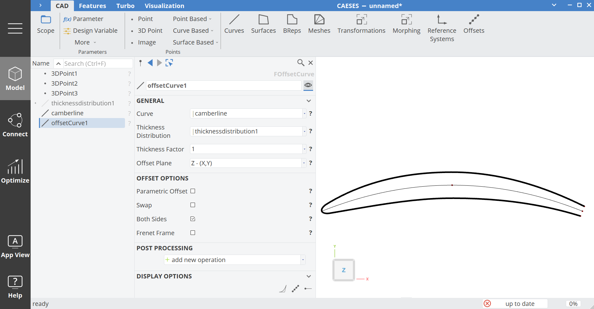
Offset curves are typically used in feature definitions to define blade sections for propellers, turbochargers and pumps.

Polycurve: Create a Single Curve

For many surface creation tasks you need to have a final single curve available. For instance, you create a sketch using 10 curves, but then you want to use the resulting single contour as input for a surface.

For this purpose, use the polycurve. It takes a set of curves and represents a single curve. You can find it in the menu

• Model > CAD > Curves > Curve Based > Polycurve.

Background Information

This is achieved by introducing repeated knots in the knot vector, ensuring interpolation at the connection points.

Important Parameter Locations

The polycurve runs within the curve interval [0,1]. However, the number of curves in the input set defines the parameter locations of the input curves within the polycurve, for the default parametrization.

For e.g. 3 input curves, the second curve start location can be found at the polycurve parameter t=1/3. The end of the second curve can be found at parameter location t=2/3. More general, the internal parameter splitting is defined by t = 1/N where N is the number of input curves.

Parametrization of Polycurves

If two curves of different arc lengths are combined with a polycurve, the parametric value t=0.5 will lie exactly at the connection point between the two curves. In some cases, this behavior may be undesirable — in such cases, switch to Unit Speed parameterization for a more uniform distribution.

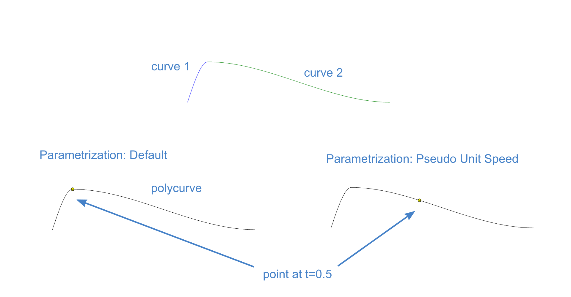
The option Start Parameter (for Closed Curves): Moves the start position (t=0) of the closed curve. The start parameter can be shifted within the range [0,1].

Auto-Orientation and Reverse

It is recommended to take care of the orientations of the input curves, i.e., make sure that the orientations are correct (all are running in the same direction, and start and end positions match correctly).

However, there is a convenient option at the polycurve to internally correct the orientations if needed called "Auto-Orientation". If checked, this option automatically reverses input curves internally to match their orientations. The end of one curve will then align with the start of the next.

Another toggle allows you to reverse the entire curve (switches the orientation).

NACA Curves

CAESES provides a set of NACA curves that you can readily use. If you need other airfoils, you can either import them through a custom import (via feature definitions), or you can directly define them in a feature definition using the mathematical description of it. You can find them in the menu

• Model > CAD > Curves > More > NACA curve
• Model > CAD > Curves > More > NACA-4DS curve.

Static Curve

In CAESES, you can create a static version of a Curve.
This is done by first selecting the desired curve and then using a Point Based Curve > NURBS or B-Spline to generate a detached curve with input points that match the selected original curve.

The resulting curve is created with fixed values for:

• Control points
• Knot vector
• (For NURBS) Weights

Since these values are fixed, the geometry is no longer connected to any parameters — it is a purely static representation.

tip

Static geometries can be used as reference models and compared against different variants of a parametric model.

Sketching

A few more comments on 2D sketching in CAESES because there is no "typical" 2D sketching functionality in CAESES as given in traditional CAD systems:

In CAESES, things follow a simple concept. You create all your curves directly in the global 3D space. If you like to be in a plane, you simply model the 3D data as needed. For instance, you would switch to a xy-view (via the 3D view button) and create a spline in the global 3D space where you set all z-coordinates of the 3D points to zero.

You can also transform contours from standard planes to arbitrary ones using image curves and transformations.

NURBS Explained

This section is designed to provide deeper insight into NURBS (Non-Uniform Rational B-Splines) curves, focusing on understanding their power and applications within CAD software. By uncovering what happens “under the hood,” this section aims to enhance your understanding and insight into using CAESES more effectively. Whether you are creating complex freeform surfaces or working with precise engineering designs, understanding these fundamental concepts can significantly improve your workflow and decision-making.

This is not a theoretical documentation - you won’t get lost in knot vector equations or spline calculus. Instead, we aim to equip you with the practical knowledge and confidence to unlock the full potential of NURBS, bridging the gap between technical power and real-world usability in CAD environments.

Why Splines Matter

Splines achieve their power through a combination of basis functions and control points, which together allow designers to shape curves and surfaces intuitively.

• Unlike purely parametric polynomial equations (which rely on abstract parameters), splines provide geometric substance that is meaningful in practice.
• Control points give designers a tangible way to manipulate geometry, making the design process more natural and interactive.

This blend of mathematical rigor and geometric intuition is what makes splines so powerful. By bridging the gap between computational complexity and human understanding, splines have become a cornerstone of modern CAD design, empowering engineers and designers to create everything from simple curves to highly complex surfaces with precision and ease.

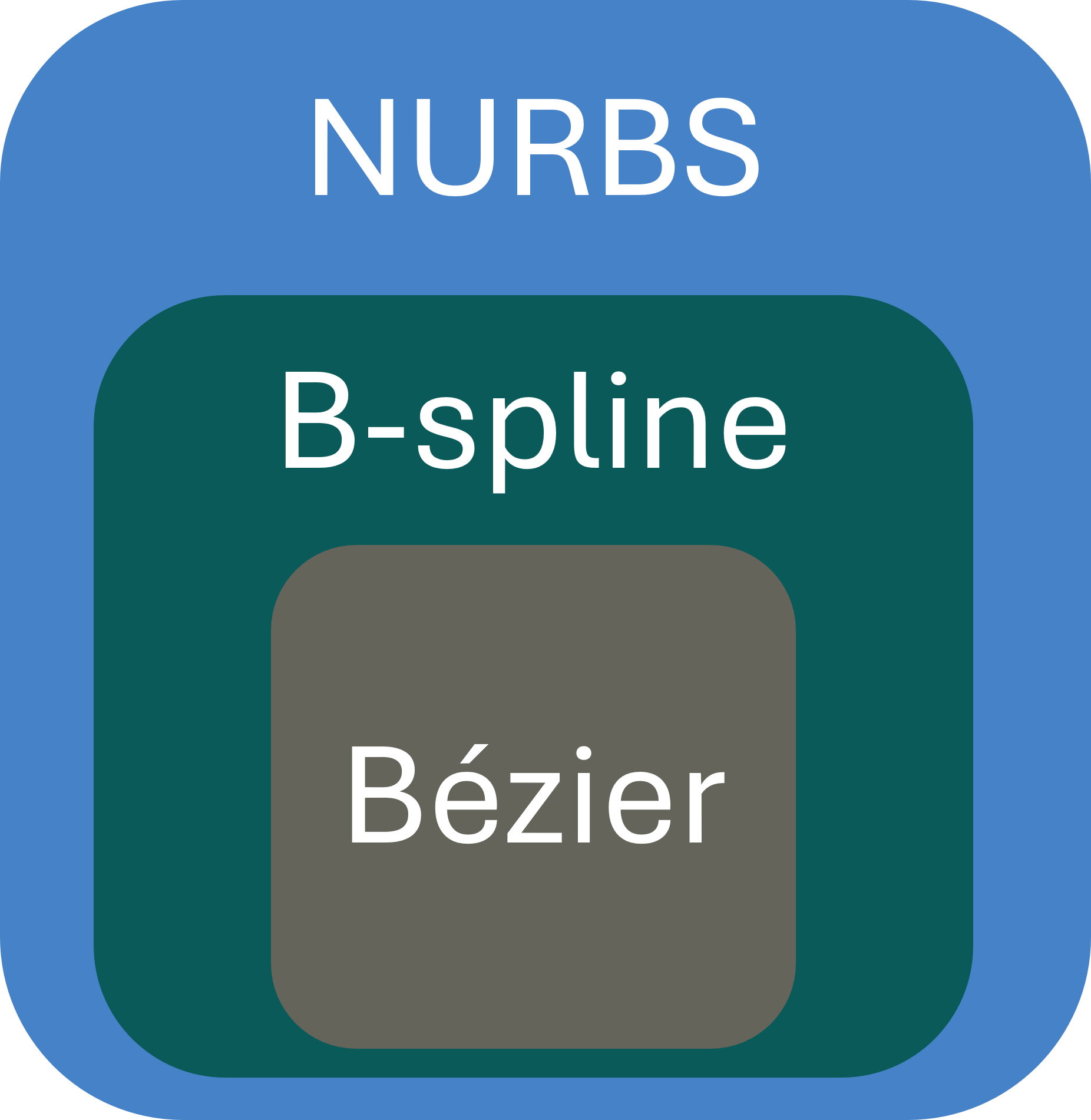
The progression of spline representations can be summarized as:

• Bézier → the simplest form, defined by control points; intuitive but limited to single segments.
• B-splines → a generalization of Bézier curves, introducing knots and multiple connected segments with local control.
• NURBS → a generalization of B-splines, adding weights to control points for exact conic sections and maximum flexibility.

NURBS (Non-Uniform Rational B-Splines) are a mathematical representation that enables the precise modeling of curves, surfaces and even complex shapes such as circles, spheres and freeform geometries.

Bézier ⊂ B-spline ⊂ NURBS

Each concept extends the capabilities of the previous one, forming the foundation of modern CAD design and freeform geometry modeling.

Practical Approach to NURBS in CAESES

This section focuses on a practical understanding of the main components of NURBS [1].

Control Points

• Control points define the shape of the NURBS curve.
• The control points do not generally lie on the curve (except at boundaries or in special cases).
• Moving a control point influences the local portion of the curve, providing intuitive control for designers.

control points

• Imagine control points as magnets that pull the curve toward them.
• In CAD modeling, always plan the distribution and number of control points:
  • Too many points → overcomplicated shapes.
  • Too few points → reduced flexibility.

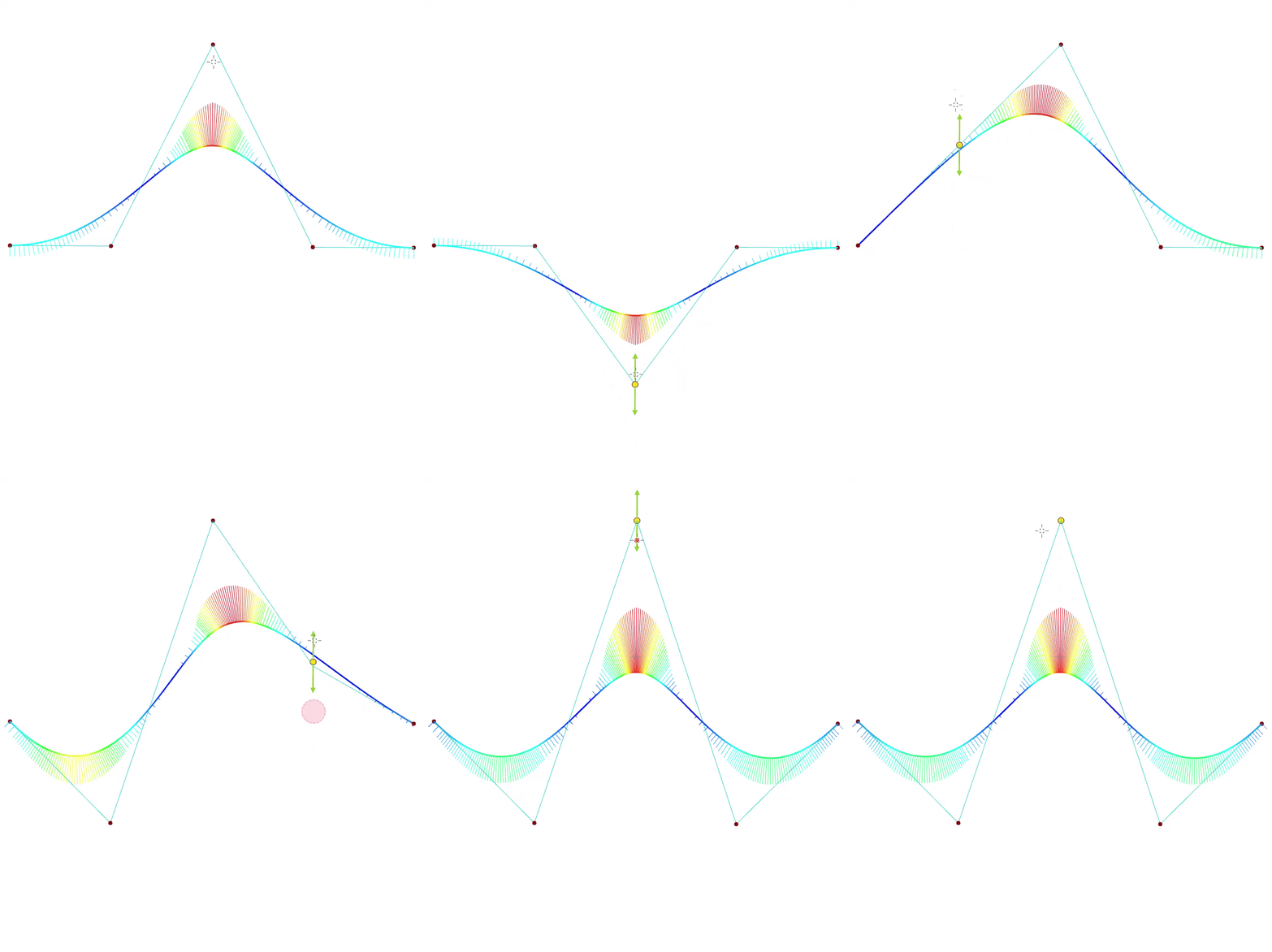Influence of control points on NURBS curve (colored spikes give an indication of the curvature)

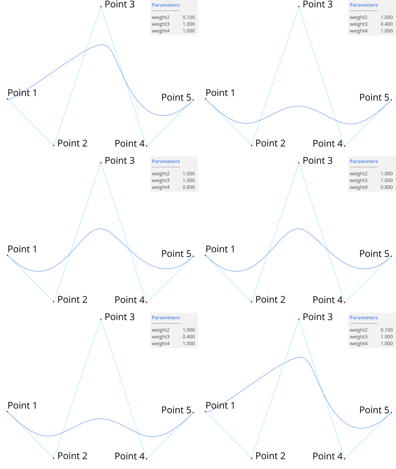
Weights

• Each control point has an associated weight that influences its “pull” on the curve.
• Higher weight → curve moves closer to that control point.
• A weight of 1 is neutral, meaning the control point behaves normally.

Weights

• Exact representation of conic sections (circle, ellipse, parabola) is possible by adjusting weights.
• Designers can fine-tune shapes locally without adding new control points.

Knot Vector

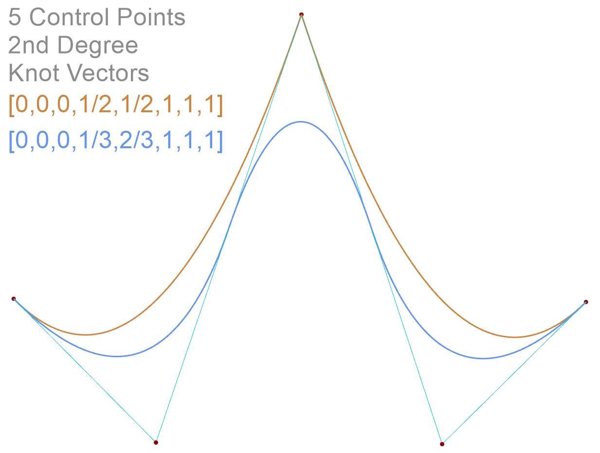
• The knot vector defines how the parameter space is mapped onto the curve.
• It is a non-decreasing sequence*of parameter values that governs:
  • Continuity (smoothness at joins).
  • Span intervals (which control points influence which portions of the curve).

Knot Vectors

• Are usually generated automatically by CAD software.
• Understanding them, however, allows custom control over parameterization and continuity.
• Uniform: knots are evenly spaced → smoother but less local control.
• Non-Uniform: knots may be repeated → enables local refinement but reduces continuity at repeated knots.
• Clamped: first and last knots are repeated → ensures the curve passes through the first and last control points.

Parameterization

• Parameterization defines how the curve is traversed along its length.
• It links the abstract mathematical formulation to the practical evaluation of the curve.
• The parameter t ranges from 0 to 1, covering the entire curve.

Parameterization

• Unit speed: parameters are spaced equally → simple but may distort the shape when control points are irregular.
• Poor parameterization can result in uneven traversal speeds and unwanted artifacts in the curve.

Degree

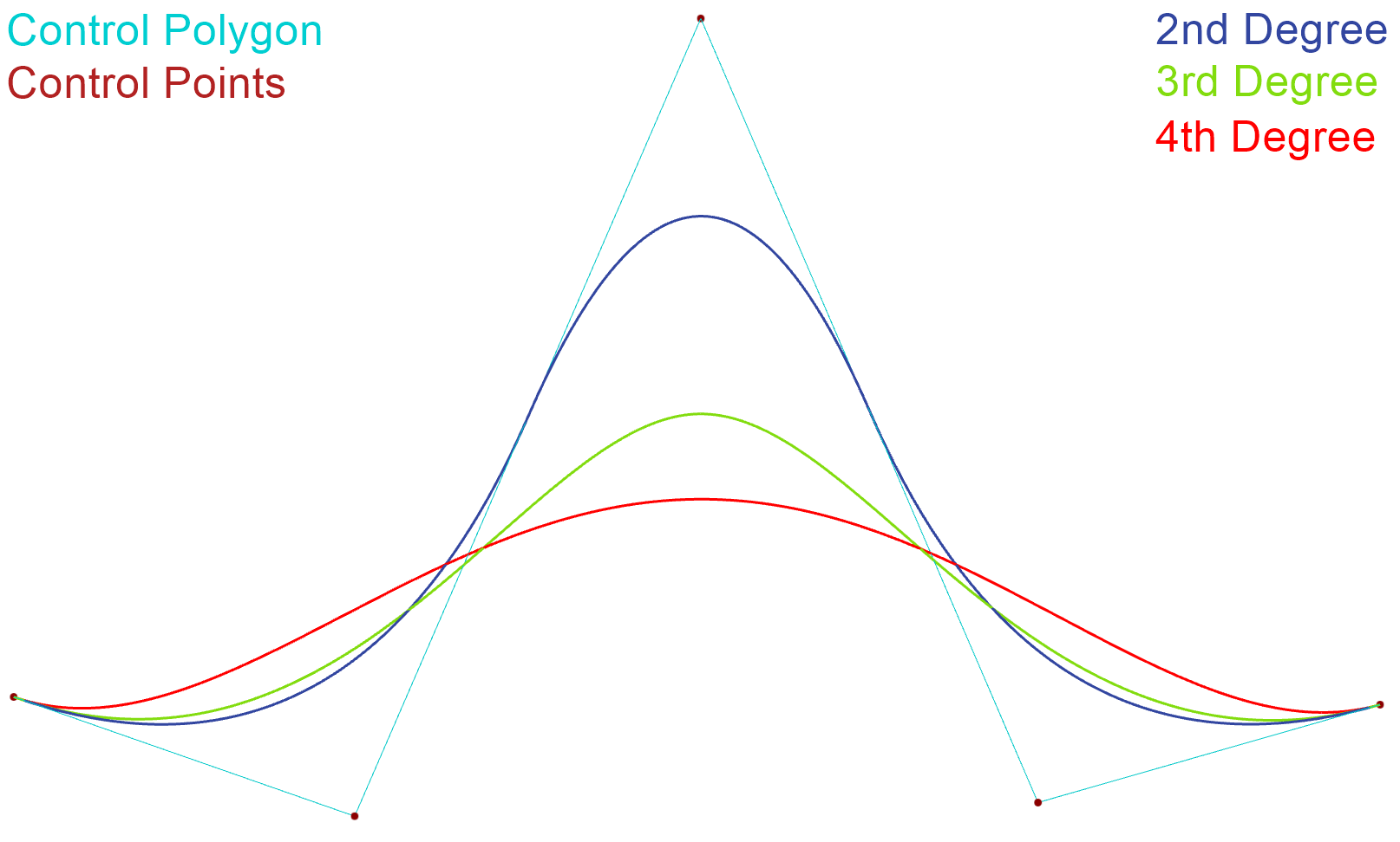
• The degree of a NURBS defines the polynomial degree of its basis functions.
• Higher degree provides more flexibility and smoothness, but also increases computational cost.

tip

• Degree 1 (Linear): straight line segments between control points with positional continuity only.
• Degree 2 (Quadratic): curves with tangent continuity.
• Degree 3 (Cubic): the most common in CAD; balances flexibility and curvature continuity.
• Higher degrees: smoother results but require more control points and computation.

Continuity

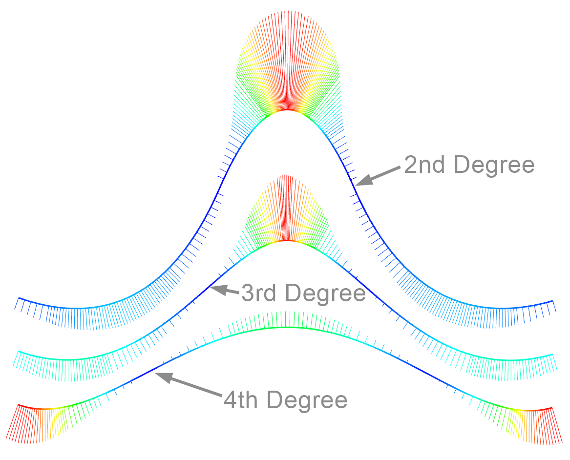
Continuity describes how smoothly two curve segments (or surface patches) connect. It is governed by the degree, knot vector and arrangement of control points.

There are two kinds of continuity:

• Parametric Continuity (C): Continuity based on the equality of derivatives of the curve’s parameterization.
• Geometric Continuity (G): Continuity based on the smoothness of the curve’s shape, independent of parameterization.

Continuity

• C⁰ / G⁰ (Positional): curves meet at the same point → used intentionally for edges and sharp transitions.
• C¹ / G¹ (Tangent): tangents match at the join → usually sufficient for engineering surfaces.
• C² / G² (Curvature): curvature matches → preferred in styling and product design for visual smoothness.

Mathematical Background

For those who want to dive deeper into the mathematics behind splines, this section introduces the core formulations of Bézier, B-Splines and NURBS.

Details

Bézier Curve

A Bézier curve of degree n is defined using Bernstein polynomials:

$$C(t) = \sum_{i=0}^{n} P_i \cdot B_{i,n}(t)$$

Where:

• $C(t)$ is the curve at parameter $t$ ($0 \\leq t \\leq 1$)
• $P_i$ are the control points
• $B_{i,n}(t)$ are the Bernstein basis functions, defined as:

$$B_{i,n}(t) = \binom{n}{i} (1-t)^{n-i} t^i$$

Properties:

• Moving a control point affects the curve globally (no local control).
• Curve always lies within the convex hull of its control points.
• Continuity: $C^{n-1}$ (global).

B-Spline Curve

A B-Spline (Basis Spline) generalizes Bézier curves by joining multiple polynomial segments, offering greater flexibility and local control.

$$C(t) = \sum_{i=0}^{n} P_i \cdot N_{i,p}(t)$$

Where:

• $C(t)$ is the curve at parameter $t$
• $P_i$ are the control points
• $N_{i,p}(t)$ are the B-Spline basis functions of degree $p$, defined recursively:

$$N_{i,0}(t) = \begin{cases} 1, & \text{if } u_i \leq t < u_{i+1} \\ 0, & \text{otherwise} \end{cases}$$$$N_{i,p}(t) = \frac{t - u_i}{u_{i+p} - u_i} \cdot N_{i,p-1}(t) + \frac{u_{i+p+1} - t}{u_{i+p+1} - u_{i+1}} \cdot N_{i+1,p-1}(t)$$

Here, $u_i$ are the values in the knot vector.

Properties:

• Local control: moving a control point affects only a limited span of the curve.
• Shape depends on the degree (p) and the knot vector configuration.
• Continuity: up to $C^{p-k}$, where $k$ is the multiplicity of a knot.

NURBS Curve

A NURBS curve extends B-Splines by introducing weights (making them Rational) and by allowing a non-uniform knot vector (hence Non-Uniform).

$$C(t) = \frac{\sum_{i=0}^{n} P_{i} \, w_{i} \, N_{i,p}(t)} {\sum_{i=0}^{n} w_{i} \, N_{i,p}(t)}$$

Where:

• $C(t)$ is the curve at parameter $t$
• $P_i$ are the control points
• $w_i$ are the weights for each control point
• $N_{i,p}(t)$ are the B-spline basis functions

Properties:

• Local control: moving a point influences only part of the curve
• Weighted control: adjusting $w_i$ pulls the curve closer to or farther from $P_i$
• Non-uniform knot vectors: enable precise control of continuity and curve segments
• Can represent both analytic shapes (e.g., circles) and freeform geometry

NURBS Surface

A NURBS surface generalizes curves into two parameters $(u, v)$:

$$S(u,v) = \frac{ \sum_{i=0}^{n} \sum_{j=0}^{m} P_{i,j} \cdot w_{i,j} \cdot N_{i,p_u}(u) \cdot N_{j,p_v}(v) }{ \sum_{i=0}^{n} \sum_{j=0}^{m} w_{i,j} \cdot N_{i,p_u}(u) \cdot N_{j,p_v}(v) }$$

Where:

• $S(u,v)$ is the surface at parameters $u, v$
• $P_{i,j}$ are the control points arranged in a grid
• $w_{i,j}$ are the weights
• $N_{i,p_u}(u)$ and $N_{j,p_v}(v)$ are B-Spline basis functions in $u$- and $v$-directions

Properties:

• Flexible representation of both freeform and exact analytic surfaces.
• Local control through grid-based control points and weights.
• Supports continuity control in both parameter directions.

References

1. Rogers, D. F. (2001). An Introduction to NURBS: With Historical Perspective. Morgan Kaufmann.