Interactive Modeling

Parametric models in CAESES are typically varied in automated studies driven by Design Engines. However, often times it is part of the preceding design process to adjust parameters and shapes by hand. Using Point Handles, Parameter Bounds and interactive expression handling this process can become very intuitive and enjoyable.

info

The beauty of this simple illustration lies in the fact that the points are parameterized (without the need to detach them for interactive dragging by their handles). One can easily imagine use cases where an initial baseline shape can be adjusted by a designer by hand and thereafter an automatic geometry variation is performed based on the already configured parametrization.

A project file with the shown examples can be downloaded here:

Load Final Model

Box Constrained Point

Let's get started with a simple example of a 3DPoint which shall be constrained in a rectangular box.

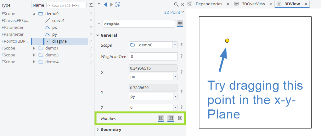
Note that under General only the x- and y-Handles are active to prevent the designer from dragging this point in z-direction. The x- and y-Coordinates are given as Parameters px and py. If you try to drag this point out of the given boundary you will notice that it always stays within the given rectangle. This behavior is achieved through bounds that are assigned to the Parameters px and py.

important

It is important to note that these bounds are allowed to hold expressions. However, converting the Parameter into a Design Variable will evaluate these expressions and set the discrete lower and upper bounds of the Design Variable based on the evaluations.

Intermediate Point

One of the fundamentals in setting up robust parametric models is to locate points relative to each other. In the following example, a point shall be at a certain relative location in between two other points. The relative position in such a scenario would typically be controlled by a Parameter or Design Variable.

While the two black points are unconstrained and their position can be chosen freely, the blue point in between is always at a relative position determined by the Parameter relPos. Again, such behavior helps to allow fast and interactive manual adjustment of a geometric model seamlessly followed by an automatic variation.

caution

Note that the correct syntax of the expressions for x, y and z of the intermediate point plays a key role in achieving the desired behavior.

I.e. writing the parameter relPos first ensures that the expression is reverse-evaluated and the parameter is automatically adjusted when dragging the point. If an expression starts with a complex term i.e. myCurve.getPos(relPos) and thus cannot be reverse-evaluated, a discrete addend will be prepended instead.

Parameter Bounds

Lower and upper bounds for the Parameter relPos ensure that it always stays within its bounds and does not "overtake" the reference points.

Circle Constrained Point

The following example is very similar to the first one, except that a circle is used as a boundary in this case. This demo is set up using two points. dragMe is meant to be the handle for the designer to work with and lookAtMe is the point of interest that shall be used in the design. The handle is constrained in exactly the same way as the Box Constrained Point earlier. However, lookAtMe will be positioned along a line connecting the origin with dragMe. The distance from the origin is calculated based on the current handle position but limited to a maximum radius by bounds assigned to the Parameter radius.

note

Notice how the handles for the two point are configured such that an inattentive user can not accidentally drag the wrong point or move the handle out of the z-plane.

3D Fillet Curve

The final example is a 3D fillet curve (tangent continuity) based on the same concepts. Two lines can be rotated freely via their end points. The tangent directions are derived and control points are located at a certain distance away from the lines. The stiffness (distance of the control points from the line ends) is parameterized and can be controlled interactively to adjust the fillet curvature according to the designers preferences. The fillet itself is a simple 3rd degree B-Spline Curve.

The absolute position of the tangent control points is parameterized relative to the distance between the two line segments as dictated by the expressions used in the Parameter bounds.

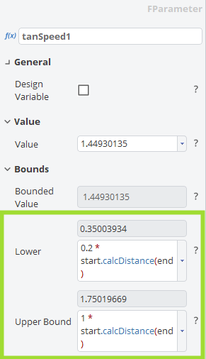
Again, it is important to note that the behavior of reverse-evaluating these expressions (i.e. automatically adjusting the Parameter value while interactively dragging a point) is dependent on the correct syntax. Generally, the Parameter to adjust should come first (and only once) followed by a mathematical operator.